Mathematica and MultiParadigm Data Science
非常功利的理由
Update:
- 2023-2-10: 参考 b 站 视频, 增加了一些函数和方法的使用情境. 更新了关于神经网络部分的一些记录.
之后要用来分析数据, 所以学一些备用.
教程是 Wolfram U 中的 MultiParadigm Data Science. 本文的作用就是用来速查的, 尽可能忠实地复制原文, 并随便添加一些注释 (在使用过后).
Update: [2023-2-10] 注: 因为这个完全是一个垃圾学习笔记, 无脑缝合了各种文档的笔记, 所以会非常的混乱且没有逻辑.
What is multiparadigm data science:
Multiparadigm Data Science is a new approach of using Al and modern analytical techniques, automation and human-data interfaces to arrive at better answers with flexibility and scale.
Build A Project Overview
This part is an overview of how the data analysis is done.
Data science projects attempt to use data to answer certain questions so that you can derive some useful insights from the answers and act on them. A flexible, modular, iterative workflow can serve as a roadmap in this quest to get from data-driven questions to actionable insights.
- Questions
- Wrangle
- Explore
- Analyze
- Communicate
Question
- What can be learned from the data?
- How many …?
- What …?
- Who …?
- Who wants to know? (which means stands at the reader's view and interests.)
Wrangle
This part is the data gathering and pre-processing, which is about gathering the data and unifying the data for further processing.
- Data Gathering 获取数据
- Pre-process 对数据进行预处理, 即:
- Beautify Data Struct 美化数据格式
- Strip Unnecessary Data 剔除不必要的数据
- Add Pivots to Important Data 增加关键的数据节点
会使用到的方法和知识:
- Key-Value Pairs 在 Ruby 里面叫做 Hash.
在 Mathematica 中为 Associations. 通过:
<| key1 -> value1, key2 -> value2, ... |>
这样的形式来组织构建.
- String Modification 字符串处理. (String Manipulation)
- StringCases Find cases of string patterns.
但是不得不说, 其形式是真的难看:
StringCases[str, patt] (* equal to StringCases[patt][str] *)
StringCases[str, lhs -> rhs] (* replace matched lhs by rhs *)
其中,
patt的规则类似于 Regexp (Ruby) (在 MMA 中也有对应 Regexp (MMA)). 简单来说是用~~连接, 用字符串 (如 =”a”= ), 字符集合 (如DigitCharacter), 匹配的函数符号 (如x_或者(x: WordCharacter)) 来组成. 使用..来表示匹配多字符.txt = "This is an example text @wolfram."; StringCases[txt, "@"~~u:(LetterCharacter | DigitCharacter | "-")..~~ (WhitespaceCharacter | PunctuationCharacter | EndOfString) :> u]
- StringReplace Make replacements for string patterns.
类似于 Ruby 里面的 String#gsub 方法.
- StringDelete 类似于查找并删除. 用于去掉非必需的字符串.
- StringCases Find cases of string patterns.
- List Manipulation 列表处理. (List Manipulation)
- Select Pick out all elements of list which
critisTrue.Select[list, crit]或者Select[crit][list]. - Sort, ReverseSort
- Count Gives the number of elements.
- DeleteDuplicates
- Select Pick out all elements of list which
- Graph and Relations 关系网络.
(Graphs and Networks, Grap Construction and Representation)
- SimpleGraph Gives the underlying simple graph from the graph.
- 一些不太好分类的
- WordCloud Generate a word cloud.
- Interpreter Something like a parser on specific rules.
比如用来处理地理数据
Interpreter["ComputedLocation"]. (注: 使用 GeoListPlot 可以在地图上输出地点, GeoHistogram 可以输出地图上的数据点的强度. )
Explore
By this stage, use the previous stage of Wrangle to visualize the data gathered and while trying to answer the questions asked at Question stage, figure out more questions of the data. (which also means returning to the Question stage)
Thus the visualization data methods:
- DateHistogram Plots a histogram of the dates.
根据日期绘制分布. 比较有用的参数:
- DateReduction 用于约化计数的范围. 传入的参数范围为 DateValue (=”Year”=, =”Month”= 等).
- Histogram Plots a histogram of the values.
比较有用的参数:
- ChartLayout Overall layout: 单参数可传入 =”Overlapped”= (重叠两张表来显示), =”Stacked”= (两张图表数值会叠在一起). 或者可以通过 =”Column”=, =”Row”= 等传入更多的参数, 但是用处感觉不是很大.
- ChatLegends 图例.
- Graph Yields a graph.
通过简单的数据处理和可视化来表现数据的性质和特征.
Analyze
To answer the question asked at the stage of Question, methods could be applied to the data.
- How many …?
- by Simply Counting
- by Comparision Charts
- by Predict the Future Data
- Predict generates a PredictorFunction based on example input-output pairs given.
- What …?
- by String Matching and Counting
- by Clustering Cluster Analysis
- by Classification (assigning labels to data)
- by Graphs and Networks (show who is connected to whom, aka,
the relationships).
- FindGraphCommunities finds communities in the graph
Communicate
Things to Remember: (How to tell the story)
- What is the story your audience is interested in?
- How can you recreate the story easily?
- Reproducible analysis
- Comparative analysis
- Easy to read and see the results.
- Easy to redo the results.
- To convince the readers.
- Notebook as an essay, report slides, cloud publishment, report template. (MMA only)
Get Your Data into Shape
This part is mainly about the Wrangle part, which could be done by:
- Handle data in different formats from different sources
- Reshape the data into different structures
- Deal with messy data
- Extract useful features from raw data
- Reduce the dimensionality of high-dimensional data
Handling Different Types of Data
Note: Before wrangling the Real-world data, you have to get them first (of course):
- Repositories of curated data
With Curated Data, it is easier to produce the data (or even skip the wrangle part.)
- Wolfram Data Repository: ResourceData Gives the primary content of the specified resource.
- Wolfram Knowlegebase: Entity Types.
- FinancialData: gives the last known price or value for the financial entity specified by name.
- WeatherData: gives the most recent measurement for the specified weather property at the location.
- Flat files
- Import Imports data from source.
And the $ImportFormats is a list of currently supported
import formats.
If passing in a URL, the
Importfunction can be used to parse the specified data format of the URL. For example:Import["https://li-yiyang.github.io/manga/animatation-review/", "Images"]
You can get a list of images (depending on your network connectivity…)

- Save appends definitions associated with a specified symbol
to a file. And DumpSave write definitions associated
with a symbol to a file in internal Wolfram System format.
After saving, use FindFile to find the file path saved. With Get (<<) can read in a file.
- Import Imports data from source.
And the $ImportFormats is a list of currently supported
import formats.
- Databases Database Connectivity
- DatabaseLink SQL Operations
Needs["DatabaseLink"]conn = OpenSQLConnection["..."] SQLTableNames[conn] SQLSelect[conn, ...] (* or, SQLExecute[] *)
- RelationalDatabase Represents schema information about a relational database.
- DatabaseLink SQL Operations
- External APIs
- comes alone Wolfram: ServiceConnect Creates a
connection to an external service, which are
listed by $Services or described at
Listing of Supported External Services.
乐, 一堆国内不好用的. - WebSearch Gives a dataset of the top web search results for the specified literal string.
- WebImageSearch Gives a list of thumbnails of the top web image search results for the specified literal string.
- WikipediaData Gives the plain text of the specified Wikipedia article.
- Publicly Available Data
- 国家统计局
不过离谱的是网站证书过期了… - China Open Data
类似一个整合网站, 不过数据不一定全部有效 - US Government's Open Data
- NASA's Open Data Portal
- UCI Machine Learning Repository
- Kaggle Data Science Contests
- Five Thirty Eight
- 国家统计局
- comes alone Wolfram: ServiceConnect Creates a
connection to an external service, which are
listed by $Services or described at
Listing of Supported External Services.
- Web scraping
吐槽
不知道该说什么好… Mathematica 难道真的是一个非常小众的东西么?
网络上的资料基本上全部都是官方的.
尽管可能是因为大家都在用… 所以比较低调?
并且连接到数据库真的好累… 可能是服务器不在国内的缘故吧.
一个曲线救国的方式就是使用梯子, 在
Mathematica -> Settings -> Internet & Mail
里面设置 Proxy Settings. 用自己的梯子来.
Restructuring Data
- Data is systematically stored
- Data elements are arranged in a structured way
from Launching the Wolfram Data Repository: Data Publishing that Really Works
吐槽
每次看 Stephen Wolfram 的博客的时候, 总有一种好像很牛逼又好像很一般的感觉. 有一种说不上来的敬佩感.
尽管有一种虽然这个问题很简单, 但是为什么要这么做的困惑. 有点像是之前计算机科学导论的课上的感觉. (尽管我那门课可能上得不太行, 但是里面的知识我觉得都是很有用的)
可能这就是牛逼的人的一种思考方式么.
Here are some helpful organized data types:
- List: List Manipulation
- Association: Associations
- Dataset: Computation with Structured Datasets
- EntityStore: Knowledge Representation & Access
- TimeSeries: Time Series Processing
Some more useful data types I think:
Lists
Most data imported are in the forms of List, and many built-in data structures (Vector, Matrix, …) are based on List.
- Read List
- First Gives the first element of exp.
And like
carandcdrin lisp (Elisp), the First function has a relative function: Rest, which gives the rest element with first one removed. - Part
expr[[]]can be used to get part ofexpr.{a, b, c}[[1]]will returna. (start counting from1, and the negative index will count backward.){a, b, c}[[2;;3]]likes python's slice, which could be written aslist[[start ;; stop ;; step]].{ {a, 1, 0}, {b, 2, 1} }[[All, {1, 3}]]will return{ {a, 0}, {b, 1} }, which could be a way to extract nested list data.
- First Gives the first element of exp.
- Process List
- List Attributes
- Dimensions Gives a list of dimensions. (kinda like giving the shape of a list)
- Length Gives the number of elements.
Associations
Associations are key-value pairs.
<|a -> 1, b -> 2|>[a]It looks more like a function written in mapping rules.<|b -> 2, a -> 1|>[[1]]will return2as the first value of it is2.- Those List functions would also work on Associations: Total, Select, Sort… (just like they are performed on the values (Values) of the associations).
- And the functions with “Key” prefixed will serve on the keys (Keys): KeySort, KeyMap.
- To map with Key-Value pairs, use AssociationMap. To construct an Association by Keys and Values, use AssociationThread and turn Association to List by Normal.
Dataset
Dataset represents a structured dataset based on a hierarchy of lists and associations.
- by Definitions
d = Dataset[{
	    <| "a" -> 1, "b" -> x, "c" -> {1} |>,
	    <| "a" -> 2, "b" -> y, "c" -> {2, 3} |>}]
- SemanticImport attempts to import a file semantically to give a Dataset object.
- by Reading
- Query row:
d[2], and rowsd[1;;2]and a row can be processed like an Association. (
d[2] // Normalwill return the Association form data) - Query with rules:
d[All, "a"]will return all the column of =”a”=.With functions passed in will be applied to the matched column. For example:
d[Total, "a"]will return the results of applyingTotalto the =”a”= column.And pass in select function will apply the function to each row:
d[SortBy[Lengh[#c]&]],d[Select[#a > 1 &], "b"](return the =”b”= column, whose =”a”= value is greater than1).And
d[GroupBy[Key["b"]], Catenate, "c"].A simple guess is that when queried with rules, functions are applied to each row and finally select the corresponding column.
- Query row:
Dealing with Messy Data
This part is fighting with the messy data, which often comes with data like:
- Incomplete
- Inaccurate
- Irrelevant
For which data cleaning is necessary:
- Replacing
- Modifying
- Removing errors
And a possible checklist for such a process can be:
- Type Checking: Consistent formatting across each row and column
- Head Gives the head of input.
- InputForm Prints as a version of
exprsuitable for input to the Wolfram Language. - DeleteDuplicates Delete all duplicates from a list. This could strip out the different types of values. Also, Sort values could help with stripping out wrong data.
- Range Checking: Reasonable and informative feature values
- Use Histogram to plot out the data to check.
- Use Select to strip out suspecious values.
- 除了上面的方法, 还可以使用统计方式来找出存在误差的值.
如: 使用正态分布来剔除 $3 σ$ 外的值, 认为在 $3 σ$ 外的值为不正常的值.
一般适合总体符合正态分布的数据, 如人口数据, 测量误差, 生产加工质量,
考试成绩等. 不适合其他分布.
或者是在箱线图中看数值是否存在异常. 比较普遍适用.
或者使用 AnomalyDetection 来生成查找非正常数据的函数. 这个处理的方式就比较无脑了.
- Missing Data: Occurrence of missing data
- DeleteCases to match values with =”NA”= missing data,
and delete them. [Note: if you have enough data to delete…]
注: 对于缺失太多的数据, 可以选择删除. 比如 40% 的缺失, 就不适合作为一个正经数据源来使用了.
- ReplaceAll (/.) Applies a rule or list of rules in an attempt
to transform each subpart of an expression
expr. [Note: Use it to replace missing value. ]The replacing methods are various:
- Replace with default values:
data /. "NA" -> 0 - Replace with means:
[Note: Also, select with Cases to provide better means.]
data /. "NA" -> Mean[Select[data, NumbericQ]]使用平均值替代的, 适用于对 个体精度要求不大, 基数大 的数据 根据定量和定性来进行区分具体使用的方法, 比如定量的数据可以考虑平均, 定性的数据可以考虑众数, 即出现次数最多的数据.
- Interpolation 插值法, 即通过构造近似函数来补上缺失值.
- 牛顿插值法: 适用于热力学温度, 地形测量, 定位等最求函数值的精确而不关心变化情况. (这个因为可能会发生振荡而不太适合求解变化的情况. )
- 样条插值法: 分段光滑曲线去插值, 连续且有连续曲率, 适用于零件加工, 要关心变化导数的问题.
- Replace with random value RandomVariate:
- Replace with default values:
First get the $μ$ and $σ$ out from good data by Mean, StandardDeviation. Then use
RandomVariateto generate.- LearnedDistribution: Guess a possible distribution.
- DeleteCases to match values with =”NA”= missing data,
and delete them. [Note: if you have enough data to delete…]
Feature Extraction and Dimensionality Reduction
This part is about extracting useful features from raw data, and reducing the dimensionality of high-dimensional data.
Feature Extraction
Transform raw data into numeric vectors to enable:
- Applying transformations like standardization, rescaling, filtering etc.
- Performing operations like Principal Component Analysis
- Calculating distances between samples
- Feeding data into Neural Networks
To extract data, the following methods could be applied:
- Nominal to Numbers: FeatureExtract and apply Feature Selection.
[Note: About the features in machine learning.]
通过
FeatureExtract来提取出数据的关键参数, 然后通过 Feature Selection 的方式来选择需要的数据以提高效率. 常见的选择方式:- Filter methods: 类似于给一个打分标准来选择什么样的 feature 更好用.
- Wrapper methods: 在数据的子集上先进行训练,
然后更换子集来看是否训练的模型是匹配的.
[Note: 可以使用 RandomSample, RandomChoice 来从数据集中提取出一个小样本. ]
[Note: 或者是对数据先 *Select* 之后再筛选. ]
- Embedded methods
Dimension Reduce
实际上也可以算是一种 Feature Extract 和 Feature Selection 的组合了.
- DimensionReduce: 自动尝试将输入进行缩减.
有一个非常炫酷的例子:
images = Import["https://li-yiyang.github.io/manga/animatation-review/", "Images"];
reduced = DimensionReduce[images, 2];
ListPlot[MapThread[Labeled[#1, #2] &, {reduced, images}]]
这个例子里面的结果就很炫酷, 可以将输入的图片直接进行一个分类. (当然, 应该不是内容识别, 猜测可能是根据图片的色调之类的进行的区分, 因为我输入的这几张图片在颜色上还是有那么一个区分的. )
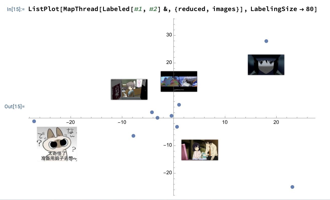
并且可以传入各种各样的参数, 所以非常的方便.
尽管都不会类似上面操作的还有 FeatureSpacePlot.
Get to Know Your Data (EDA: Exploratory Data Analysis)
What to do at this stage:
- Gain an intuitive understanding of the underlying nature of the dataset
- Identify relationships between variables
- Formulate good questions for the actual analysis (as the explorations proceed, those questions can change)
- Evaluate the quality of data (Data QA)
Questions to keep in mind for EDA:
- Do we have the data as needed for the planned analysis? Is there enough of it?
- Does the data seem to be accurate? Are there obvious errors? Is the data missing something?
- Is the data relevant? Are there outliers?
- Are there some characteristics of the features that attract attention right away?
EDA Checklist:
- Visualise the data in feature space
- Try pairs of raw features
- Project data to 2 or 3 dimensions through Dimensionality Reduction.
- Create scatterplot matrices to look at pairwise relationships across all variables
- Plot distributions of all variables
- Start with single distribution - single variable
- Go on to joint distributions of pairs of variables
- Overlay plots and graphs
- Compare distribution shapes to histograms
- Look for deviations
- Visualise clusters of samples
- Identify outliers
- Look for gaps in the data
- Plot time series data to identify trends
- Try visualization tools from other disciplines
- Look at pairwise relationships between variables - correlation
Visual Exploration
We are visual creatures. Visual things stay put, whereas sounds fade.
人是视觉的动物.
by Steven Pinker
所以数据可视化对于认识数据极其有帮助.
Tools of EDA:
- Graphical (visualizations) or Non-graphical (statistics)
[Note: a useful website about Visualization Plots. ]
- Show 用于整合输出多幅图
- Scatterplots (散点图) ListPlot
通过 Grid 来组织不同的图表来展现不同类别的散点图.
- BarChart (柱状图, 相对大小), PieChart (饼状图, 成分占比)
- Histogram, 或使用 PairedHistogram 来进行对比.
注: 一个绘图的小技巧是在绘图前可以对数据进行一个缩放 Rescale, 使得其输出结果更加容易看:
dataScaled = With[{
        dat1 = ({Min[#1], Max[#1]}&)[dur],
        dat2 = ({Min[#1], Max[#1]}&)[wait]},
             (Rescale[#1, dat1, dat2]&) /@ dur];
上面是来自官方的代码, 满满的函数式编程的味道.
其他的还有: DensityHistogram, Histogram3D, SmoothHistogram, SmoothHistogram3D.
- BoxWhiskerChart (箱线图)
注: 箱线图的 (线) 两端表示最大和最小, 中间的框表示第一四分位数, 第三四分位数的一个范围. 最后中间的线表示中位数. 其反应了数据的: 中心位置, 散布程度, 对称性的信息.
可以用箱线图来帮助了解数据是否有误. 如从上下极限可以找到是否有异常数值, 或者根据四分位距 $IQR = Q_3 - Q_1$ 来判断, 再通过设置一个合理区间来判断. 即设置上极限和下极限的区域为 $Q_1 - 1.5 × IQR, Q_3 + 1.5 × IQR$. 是一种比较普遍适用的方法.
- DistributionChart (默认) 得到的是 Violin Plots (小提琴图).
注: 类似于箱线图的升级版本. 可以和人口年龄结构分布图类比一下.
- QuantilePlot (Q-Q 图)
注: 用来表示两个分布之间的差异. 比如默认是和标准分布的差: 假设数据样本的概率分布为 $F(X)$ 而标准分布为 $\hat{F}(X)$. 那么如果将其差 $F(X) - \hat{F}(X)$ 在一条直线附近绘制出来, 就会得到 Q-Q 图.
- Do two data sets come from populations with a common distribution?
- Do two data sets have a common location and scale?
- Do two data sets have similar distributional shapes?
- Do two data sets have similar tail behavior?
- Cluster visualizations 通过对数据进行分类以达到数据可视化的程度.
- FindClusters 对输入的数据进行一个分类
- ClusteringTree 基于树状图的一个分类, 类似的还有 Dendrogram 来绘制.
- TimeSeries plots
- WordCloud
[Note: 可以用来分析词条的出现频次.]
- Univariate (single variable behavior) or multivariate (combined behavior of two or more variables)
Looking at Data Differently
这一部分的想法就是, 对于不同的类型的数据, 通过不同的方式来处理, 可以得到很好的结果:
- 词条的出现频次, 通过 WordCloud 这样的方案就很好
- 对于低维数据, 可以通过简单的绘图的方式显现.
但是对于复杂的高维数据, 则可以通过特征提取的方式来分类.
- FeatureSpacePlot
- Graph, and HighlightGraph helps information stand out.
- 对于特定的种类的数据, 可以用专门的方式来绘制:
Statistical Tools
- $\bar{x} = ∑ x_i / N$ Mean, $∑(x - \bar{x})^2/N$ Variance
- $σ$ StandardDeviation
- Tukey's Five number summary
注: 这个 Five number summary 描述的量在箱线图中就有表述.
- Frequency Counts Count
[Note: when dealing with *Float* data, it is helpful to first apply Round.]
- Correlation
- Others
Assenble a Multiparadigm Toolset
This part is about using tools to answer the questions asked above.
Quick Review of Terms: (黑话介绍)
- Independent variables as input $\vec{x} = {x_1, …, x_n}$
- Dependent variable as the result $y$.
- Model about how input generates the output, which could be a function $y = f(\vec{x})$ or just simply a blackbox: $\vec{x} → \mathrm{blackbox} → y$.
- Parameters are values in the model or algorithm that are not assumed by the predictor or response variables; learned/tuned while training.
- Training The process of identifying the function or the algorithm (and the corresponding parameters) that best represents the relationship between the input and output.
Classification
This part is about answering the question like Is this A or B?
Use Classify to mark data, return a ClassifierFunction which could classify input. The ClassifierFunction can be used for getting the probabilities for all classes or a specific class.
c = Classify[data];
c[value] (* Return the class *)
c[value, "Probabilities"] (* All possible classes with probability *)
c[value, "Probabilities" -> "A"] (* Probability for a specific class*)
思路是这样的, 在数据集中选择一个代表数据集, 然后进行手工标定, 最后用 Classify 来对数据集进行学习, 以期望能够通过学习的结果, 用来对其他的数据进行预测.
训练的方法 Classify[data, Method -> "..."] 有: (方法内容介绍有空补)
- Logistic Regression to classify using probabilities from linear combinations of features.
- Nearest Neighbors to classify from nearest neighbor examples
- Naive Bayes to classify by assuming probabilistic independence of features
- Decision Tree to classify using a tree-like model for representing decisions and their consequences
- Gradient Boosted Trees to classify using an ensemble of trees trained with gradient boosting
- Random Forests to classify using Breiman-Cutler ensembles of decision trees
- Markov Models to classify using a stochastic model on the sequence of features (for text, bags of tokens, etc.)
- Support Vector Machines to classify using a discriminative model that constructs a hyperplane or sets of hyperplanes to separate samples of different classes.
- Neural Networks to classify using algorithms modeled loosely after biological neural networks.
- 更多方法见 Classify 文档.
训练结果可以添加用来判断分类的阀值, 如:
Classify[data, IndeterminateThreshold -> 0.9`],
若没有高于阀值的分类结果, 则返回 Indeterminate 表示不能判断.
也可以在实际使用中添加参数: cfunc[value, Indeterminate -> ...].
在训练的时候, 可以传入标定概率的数据集 UtilityFunction 来增强分类结果.
utility = Association[
  "a" -> Association["a" -> 1, "b" -> 0, Indeterminate -> 0.5`],
  "b" -> Association["a" -> -15, "b" -> 1, Indeterminate -> 0.8`]];
ClassifierMeasurements[c, test, "ConfusionMatrixPlot", UtilityFunction -> utility]
使用 PerformanceGoal 参数在 Classify 中可以改变分类的性能.
是速度优先或者是质量优先或者其他.
对于结果, 通过 Information 来提取关于拟合的 ClassifierFunction 函数的信息,
比如 Information[c] 得到所有关于 c 的信息. 或者再传入一个参数指定信息:
Information[c, "MethodOption"]. 其中的参数还有: LearningCurve (训练曲线),
Accuracy 精确度等等.
使用 ClassifierMeasurements 来评估一个 ClassifierFunction 的好坏程度.
其中, test 为另一部分人为标定的数据集. cfunc 是根据部分标定的数据训练得到的结果.
cfuncMeasure = ClassifierMeasurements[cfunc, test]
cfuncMeasure["Accuracy"]
cfuncMeasure["ConfusionMatrixPlot"]
其中的参数有:
- Accuracy: fraction of correctly classified examples
- ConfusionMatrixPlot: plot of the confusion matrix
- BestClassifiedExamples: examples having the highest actual-class probability samely: WorstClassifiedExamples.
总结:
- Classification as a supervised machine learning task of predicting labels for new samples, based on a set of previously labeled training samples
- Classify: a machine learning super-function
- Works for various types of input–numerical features, images, text, etc.
- ClassifierMeasurements: to evaluate the performance of the ClassifierFunction created by Classify
- Customize Classify to:
- Use different “Methods” or common classification algorithms like Logistic Regression, Decision Trees, Nearest Neighbor etc.
- Use different UtlityFunction and IndeterminateThreshold for making decisions
- Optimize performance according to different criteria like training speed, actual runtime speed, memory usage, or accuracy of predictions
Regression
This part is to answer How much would something be.
- Linear Regression LinearModelFit
lm = LinearModelFit[data, {f1, f2, ...}, {x1, x2, ...}]
lm["BestFit"] (* linear exp of f1, f2, ... *)
- Machine Learning Super Function Predict
PerformanceGoal- Methods used to generate prediction:
BoostingMethod
- Test of predicted results:
- Plot distribution of predicted function on specific input:
Plot[PDF[predictFunction[input, "Distribution"], x], {x, 0, 1}] - PredictMeasurements to test predicted results.
ComparisionPlotto plot predictions with data input.StandardDeviationReport
- Plot distribution of predicted function on specific input:
FindFormulato find a formula to describe the given data
Cluster Analysis
The previous two parts use a lot of supervised machine-learning methods. This part is about some unsupervised machine learning methods, which will answer questions like:
- How is the data organized?
- Does the data have some inherent structure?
- Do the samples sort themselves out into different groups and subgroups?
FindClusters 来对输入的函数进行分类. 其中可以传入的参数:
DistanceFunction对于输入的一个距离函数, 需要满足的条件: $f(e_i, e_i) = 0, f(e_i, e_j) \geq 0, f(e_i, e_j) = f(e_j, e_i)$.默认使用的距离函数根据不同的输入会有不同的结果. 如对于 Numeric data, 可以是 Euclid Distance; 对于 Boolean data, 使用的方法是 Matching Dissimilarity or Jaccard Dissimilarity; 对于 String data, 方法为 Edit Distance 或 Hamming Distance.
Nearest 函数用来找最近的元素.
Nearest[list, query, <number>]. FeatureNearest, FeatureSpacePlot.Method用来指定使用的分类方法CriterionFunction
其他类似的函数有 ClusteringTree, Dendrogram, 以及 ClusteringComponents 可以给出不同元素所对应的类别的一个 list.
ClusterClassify 函数可以通过使用 Cluster 的方式来构建一个分类函数.
LearnDistribution 和 FindDistribution 的作用和 FindFormula 类似, 可以根据输入来生成一个可能的分布.
Anomaly Detection
Answer the question about is this unusual?. To perform anomaly detection, here are some methods:
- Network instrusion
- Fraudulent transaction
- Unusual characteristics of diseased cells
AnomalyDetection 可以在样本的基础上训练一个找不同函数,
配合 FindAnomalies 函数使用可以在输入中找到一个不同的函数结果.
后者通过传入 AcceptanceThreashold 参数来改变默认的剔除阀值.
这个找不同函数也可以用来 DeleteAnomalies. 来防止不同的样本对后续分析的影响.
或者是使用 LearnDistribution 生成一个分布, 并使用 RarerProbability
来找出那些不太可能出现的量 (通过概率来). 并且可以用这个生成的分布,
来填补之前的 Missing 的数据. 使用的函数是 SynthesizeMissingValues.
Predict of Next Value
Use SequencePredict to generate a SequencePredictFunction,
which could be used to generate the next value of input by learning
sample data: predictFunc[input, "RandomNextElement" -> num].
在 SequencePredict 使用不同的参数来处理输入:
FeatureExtractor来指定如何提取输入的关键部分, 如SegmentedWordsMethod中可以指定Markov链的长度Method -> {"Markov", "Order" -> 5}, 类似这样.
灰色预测模型 $GM(1, 1)$
适用于时间序列预测, 灾变预测, 波形预测, 系统预测. 其中 $GM(1, 1)$ 表示仅含有一个变量的一阶微分方程模型.
Neural Networks
The good news is that the Wolfram Neural Net Repository and the Neural Net Framework in the Wolfram Language makes it really easy to incorporate this powerful technology into our project workflow.
The bad news is that we could never do justice to covering this topic in just 10 minutes.
- Neural networks are either chains or (acyclic) graphs of layers
- Layers process arrays (a.k.a. tensors) of numbers (a.k.a. neural activities)
- Encoders and decoders convert the input to and output from numerical arrays
- Frameworks provide different loss functions
- Frameworks provide built-in backpropagation and stochastic gradient descent
- Frameworks are highly optimized to run on (special) hardware
所以关于神经网络的部分还得之后继续学.
可以参考的网站:
- WOLFRAM NEURAL NET REPOSITORY
- Perform Net Surgery for Transfer Learning
- Introduction to Neural Nets
- 动手学深度学习 (但是不是 Mathematica 的版本)
Introduction to Neural Networks
Introduction to Neural Networks
课程是 Wolfram U: Introduction to Neural Networks 的课程.
What are Neural Nets?
Modertn term: differentiable programming (wikipedia).
Layers (Operator)
[Note: 因为我是照着英文从零开始学的, 所以并不知道名词应该怎么翻译. 故以下名词全部保留英文. ]
Layer 是一个网络中最基本的组成, 类似于一个运算子 (operator), 但是只接受数值输入的 tensors:
elem = ElementwiseLayer[Tanh];
{elem @ {1, 2, 3},
N @ Tanh @ {1, 2, 3}}
{ {0.7615941762924194, 0.9640275835990906, 0.9950547814369202}, {0.7615941559557649, 0.9640275800758169, 0.9950547536867305} }
且 Layer 是可导的. (可导性为后续用于计算参数 “学习” 的一个前提. )
elem[{1, 2, 3}, NetPortGradient["Input"]]
D[Tanh[x], x] /. x -> {1., 2., 3.}
其他关于 Layers 的一些知识
在运算的时候可以指定 GPU 和 CPU 来进行运算:
elem[{1, 2, 3}, TargetDevice -> "GPU"]
注: macOS 貌似没有对 GPU 的支持.
[等一下, 我突然发现讲课的人用的是 macOS, 且其 GPU 至少有 3 线程… 是我的电脑不配么…]
在新建 Layer 的时候可以指定输入的类型:
ElementwiseLayer[Tanh, "Input" -> {4, 32}]
上面的就是一个 $4 × 32$ 的矩阵作为输入.
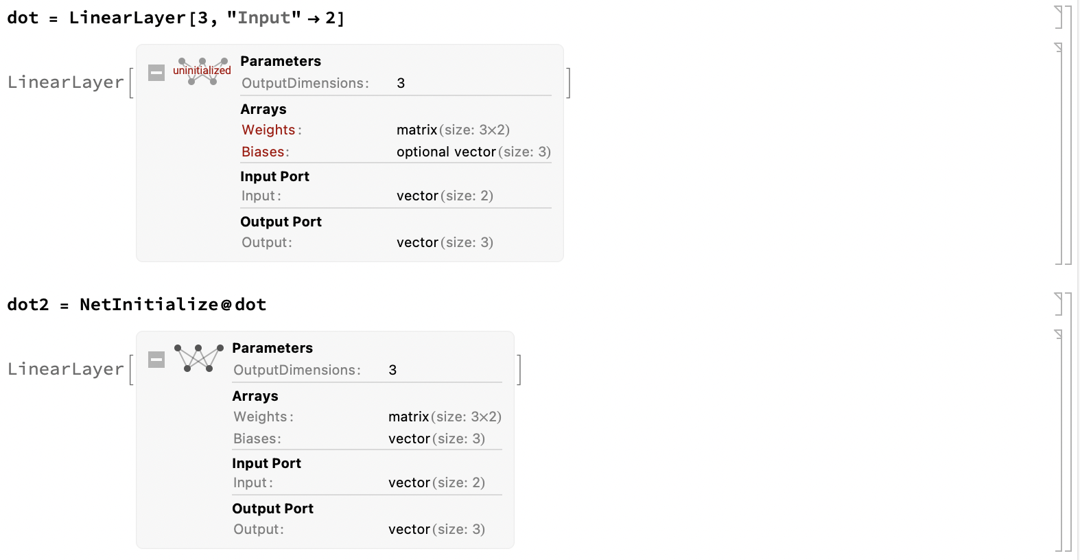
一些 Layer 有可学习的参数:
dot = LinearLayer[3, "Input" -> 2]
注: 上面的是一个三维输出, 二维输入的一个线性 Layer.

而默认是没有初始化这些未知的参数的, 所以需要通过初始化的方式 (NetInitialize) 来给一个 Layer 赋上随机的参数值. 使用 NetExtract 可以提取出参数的具体值.
通过 ?*Layer 可以列出可用的各种 Layer.
Chain and Graph
使用 NetChain 可以将多个 Layer 串联在一起, 将其输入和输出依次相连. 但是这样得到的只是单输入的一个网络. 使用 NetGraph 可以构建有多个输入的网络.
比如有一个函数是: func = (Tanh @ #Input1 + LogisticSidmoid @ #Input2)&,
用网络来表示就是:
NetGraph[{ElementwiseLayer[Tanh], ElementwiseLayer[LogisticSigmoid], TotalLayer},
{NetPort["Input1"] -> 1, NetPort["Input2"] -> 2, {1, 2} -> 3}]
其中 1, 2 对应的就是第一个参数 (节点列表) 中节点的顺序.
于是对于这样的 net, 通过 net @ <| "Input1" -> {...}, "Input2" -> {...} |>
的形式来进行计算.
NetEncoder and NetDecoder
使用 NetEncoder 可以对输入的数据进行一个解码. 如对输入的图片以灰度形式转换为 $12 × 12$ 的一个张量:
NetEncoder[{"Image", {12, 12}, "ColorSpace" -> "Grayscale"}]
参考文档:
或者可以直接通过 *Layer[..., "Input" -> NetEncoder[...]]
来指定一个 Layer 输入的类型.
使用 NetDecoder 可以将张量转换为原始的输出.
通过 *Layer[..., "Output" -> NetDecoder[...]] 的形式,
可以来指定一个 Layer 输出的类型.
Training
使用 NetTrain 可以根据输入的数据来训练一个网络.
一个输出的数据的例子如下: {input -> output, {1, 2} -> 3},
类似这样.
其使用 Gradient Descent (梯度下降) 的方式来对参数进行查找. 但是其原理目前并不需要太过了解.
An Example: a Digit Classifier
详细的介绍在 Notebook 里面可以查看. 简单的介绍如下:
- 使用 LeNet 来构建的神经网络, 主要包含的内容如下:

[Note: 图片来源: 动手深度学习: LeNet ]
- 使用一个 NetGraph 来用于训练.
注: 最终训练的网络结果可以在 这里 下载.
Get the Message Across
Visualizations
列举一些绘图用的函数以及其可能的用途和参数:
[Note: 因为这些参数并不只能用在一个函数中, 其他函数估计也可以, 但是这里只记录一次出现. ]
- BarChart 柱状图, 用于表现各组分的数量比较关系
- ChartLabels 用于给组分进行标记, 一个比较妙的标记方式:
ChartLabels -> Keys @ data对于绘制的 Label, 默认是在下方 (x 轴), 通过
Placed[Keys @ data, Top], 可以放在柱的顶部. 通过Callout[Keys @ data, Above]可以以箭头注记的方式标在顶部. - AxesLabel 用于绘制坐标轴上的注记 (轴末端, 水平方向), 类似的还有 FrameLabel (框线侧, 框线方向) 和 Frame. 后者通过布尔值来判断是否在图的四周绘制框线.
- PlotLabel 用于绘制图顶部的图名称
- PlotTheme 用于标记图表的主体, 类似的有 ChartStyle, PlotSytle. 区别在于 PlotTheme 改变的是图表的数据标记, 框线之类的非主体要素; ChartStyle 改变的是图表绘制的内容 (柱条颜色) 之类的主体内容整体指定; PlotStyle 则是对每一个元素主体进行一一指定.
- ImageSize 指定绘制的图表的大小
- ChartLabels 用于给组分进行标记, 一个比较妙的标记方式:
- RectangleChart 可以用来绘制二维向量的柱状图, 每个矩形的横宽和竖高分别代表不同的向量的分量.
- BubbleChart (泡泡图?) 可以用来绘制三维向量的图,
用在 $xOy$ 平面上半径为 $r$ 的不同大小的圆来表示 $\{x, y, z\}$ 这样的向量.
类似的还有 GeoBubbleChart.
- ChartLegends 给出图例
一个比较适合多数据的颜色的图例为 BarLegend. 这个函数适合配合 ChartStyle 一起使用, 如:
ChartLegends -> BarLegend[{<ChartStyle>, QuantityMagnitude[MinMax[data]]}] - Tooltip 一个对于导出图片来说没什么鸟用的 Mathematica Notebook 限定的华丽操作. 可以指定在 Mathematica 绘制出来的图片上, 当鼠标放置在特定元素上时, 弹出的自动提示框的样式.
- ChartLegends 给出图例
- Manipulate 可以用来给图表添加交互性, 也是一个 Mathematica Notebook 限定的华丽操作. 像 Mathematica Engine 这样的就无福享受了.
- 对数坐标轴, 有助于将中间的对象提取出来, 防止挤在一起
- Graph 关系图
一个非常酷的关系图的例子:
data = (* a list *)
nearby = Flatten[Map[(Thread[# -> DeleteCases[Nearest[data, #, 3], #]])&, words]]
Graph[nearbys, VertexLabels -> Automatic]
或者用 NearestNeighborGraph 也可以实现类似的功能.
一个更加炫酷的例子:
wordPlot[w_String] := Graph[(x = Characters[w];
  Thread[Drop[x, -1] -> Drop[x, 1]]), VertexLabels -> Automatic,
  DirectedEdges -> True];
wordPlot["Shakespeare"]
更多参考: Data Visualization 或者 Data Visualization with the Wolfram Language. Visualization and Graphics.
Automated Reports
自动化一键生成报告, 很好. 不过因为不太能用到, (平时以 Org-mode 为主), 所以这部分快速一点:
- CreateDocument 用来生成一个最终的文档
- CreateNotebook 配合
CreateNotebook["Template"], 用于生成模版.
Microsites and Web Apps
因为 CloudDeploy 要 Credits, 所以这部分就是穷鬼看看就好了.
其中将计算的结果用 iframe 的形式嵌入到网页中这个功能我觉得是可用的,
不过可能需要有一些更加实际的场景才能让穷鬼花费自己的 Credits 去部署吧.
Reproducible Research Checklist
这个我觉得很有必要, 可复现性.
Publishing data-backed reproducible analyses enable the community to:
- Verify results (Replication == Stronger evidence)
- Build on existing results
- Combine results for better insight
为了达到上面的目的, 一个 checklist:
- Build a flexible, modular iterative workflow in stages (Question, Wrangle, Explore, Analyse, Communicate)
- Plan for structured data analysis
- Automate (write code) the process wherever possible. (Avoid point and click).
- Document the code; Use a notebook-based workflow to combine code and visualizations along with text descriptions (styled and formatted for better communication)
- Record and preserve
- Sources: raw data, goals, references
- Process: explorations, final code, observations, and comments (selections and rejections)
- Output: clean data, visualizations, reports, apps
- Use version control
- Prepare for obsolescence - things will change, and sources will get removed. (存档或者对新资源重新利用)
Other Mathematica Functions
因为官方的教程中大量使用了 Mathematica 中的缩写和函数式的知识, 所以在这里进行一个记录以用来之后的查找.
- With, 使用方法就像是 Lisp 中的
let方法. 提供临时局部变量绑定. 但是并不能做到按顺序进行依次赋值, 比如With[{a = 1, b = a + 1}, exp]这样的表达式是不能够实现的. 可以通过嵌套的With来曲线救国. - 函数 Function: 定义一个完整形式的函数
Function[arg, exp], 如Function[{x, y}, x + y]生成一个函数. (和 Lisp 中的(lambda (arg) exp)类似)或者使用缩写形式:
(exp)&来表示一个表达式, 其中用#,##,#1,##2这样的方式来表示传递进来的参数. 其中:#形式代表选择对应的传入参数, 默认为第一个参数, 带上数字后缀则表示对应的位置的参数, 比如#1为第一个传入的参数,#2为第二个传入的参数, 依此类推. 比如(#1 ^ #2)&[2, 3]就会变成2 ^ 3.##形式代表选择从某一位开始之后的传入参数, 默认从第一个参数开始, 带上数字后最则表示从对应位置开始的所有参数, 如##2为从第二位开始的所有参数. 比如(##2)&[1, 2, 3, 4, 5]就会返回Sequence[2, 3, 4, 5]. 比较少用.
- Map 系的函数: Apply (相关函数: Evaluate), MapThread, MapIndexed 等.
一些简单的例子和缩写:
(#^2)& /@ Range[5]  (* Abbrevation of Map[(#^2)&, Range[5]],
                      but Table[i^2, {i, 5}] is better. *)
MapThread[(#1 -> #2)&, { {a, b}, {1, 2} }] (* Return {a -> 1, b -> 2} *)
MapIndexed[f, {a, b}] (* Return {f[a, {1}], f[b, {2}]} *)
其他的参考:
Functional Programming Quick Start
参考 Wolfram U 上的 Functional Programming Quick Start 课程.
- Everything is an Expression
除了基本的元素以外, 所有的 Mathematica 中的表达式的形式都可以归化为
Head[elem1, elem2, ...]的形式. 而一些操作符号有其对应的缩写形式 (shorthand). - Evaluation of Expressions
使用 Attributes 可以查看函数的特性, 譬如对于 Plot 函数,
Attributes[Plot]的返回值为{HoldAll, Protected, ReadProtected}. 其中Protected表示被保留, 不会被随便写掉. 而HoldAll表示Plot不会将其参数先执行求值后运算. (类似于 SICP 中的 applicative-order 和 normal-order 的感觉. ) - List, the Functional Workhorse
- Procedural to Functional Programming
Mathematica is a multi-paradigm language, and while procedural programming is supported, it is better to use the system using its native paradigm.
- Lose the Loop:
Do[exp, {iterVar, start, end}], 但是效率不高, 所以并不推荐. 一般的历遍和建表的操作, 应该选用 Map 和 Table. - Conditional Programming:
If[condition, t, f], 或者是缩写形式t /; condtion.- 或者是
func[var_?EvenQ]这样的 pattern 形式. 这样的形式可以用来替换Which的分支定义:func[n_] := Which[cond1, exp1, cond2, exp2] (* The following are equal definitions *) func[n_?cond1] := exp1; func[n_?cond2] := exp2;
- Lose the Loop:
- Patterns and Rules
About Mathematica And Emacs
- A helpful guide about mathematica and emacs can be seen here.
You may need first download ob-mathematica.el to your included path. And at line 34, change
(org-babel-get-header params :var)to(org-babel--get-vars params)according to this issue.And using mash.pl can help with evaluation.
- And a mathematica LSP server can be seen at Github:
WolframResearch, or lsp-wl, which need to write yourself
emacs code. (I choose the latter one.)
Although I can't tell why it was slow to connect. - To enable lsp-mode for org-src-mode when editing Mathematica code, could refer to this issue. (which I think is important, especially for something like Mathematica with tons of functions.)
- Also, you can use Jupyter and Wolfram Engine, which, I think is a bit complicated.
Others
All models are wrong. Some are useful.
线性规化, 非线性规化和多目标规化 - 最优方案
线性规划
对于 线性规化 的问题, 若有不等式方程组为条件:
$$\left\{\begin{array}{lll}x_1 + x_2 & \leq & 6 \\ x_1 & \geq & 1 \\ x_2 & \geq & 1 \\ 240 x_1 + 120 x_2 & \leq & 1200\end{array}\right.$$
想要求 $y = 40 x_1 + 30 x_2$ 的最大值.
使用 LinearOptimization 方法来计算最小值时的变量取值.
LinearOptimization[ - (40 x1 + 30 x2),
  {x1 + x2 <= 6, x1 >= 1,  x2 >= 1,
     240 * x1 + 120 * x2 <= 1200}, {x1, x2}]
{x1 -> 4, x2 -> 2}
或者直接扔到 Minimize 或者 Maximize 函数中可以得到结果:
Maximize[{40 x1 + 30 x2,
          x1 + x2 <= 6 && x1 >= 1 && x2 >= 1
          && 240 * x1 + 120 * x2 <= 1200},
  {x1, x2}]
{220, {x1 -> 4, x2 -> 2}}
并且上面的 Minimize 和 Maximize 方法还不只适用于线性规划:
NMinimize[{x1^2 + x2^2 + x3^2 + 8,
  x1^2 - x2 + x3^2 >= 0 && x1 + x2^2 + x3^2 <= 20 &&
   -x1 - x2^2 + 2 == 0 && x2 + 2 * x3^2 == 3 &&
   x1 >= 0 && x2 >= 0 && x3 >= 0}, {x1, x2, x3}]
{10.651091807695447, {x1 -> 0.5521673359041438, x2 -> 1.2032591743672956, x3 -> 0.9478240343844963}}
注: 并不适合多变元的问题. (参考)
其他的方法有二次规划 (QuadraticOptimization), 罚函数法, 梯度法等, 可以参考文档:
多个目标规划
- 每个目标都有一个完成情况的目标 $d_i^0$,
- 取实际值函数 $f_i$, 于是可以得到正偏差 $d_i^+ = max\{f_i - d_i^0\}$ 以及负偏差 $d_i^- = -min\{f_i - d_i^0, 0\}$.
- 绝对约束是前提的约束, 而目标约束是对目标的一个要求,
类似于绝对约束是客观事实, 而目标约束是画的大饼应该有的样子,
比如利润目标应 $f_i \geq 2,000$ 之类的. 目标约束可以有一定的偏差,
于是可以加入正负偏差变量: $f_i + d_i^- - d_i^+ = d_i^0$.
注: 上面的偏差公式的意义是: $f_i$ 可以比 $d_i^0$ 小 $d_i^-$, 可以比 $d_i^0$ 大 $d_i^+$. 如果一个目标约束只能偏大, 那么就不能有 $d_i^-$ 的项.
好处: (为什么这样做), 将偏差用正负偏差变量来代替, 可以把目标函数变成等式的约束条件. 等式的约束条件也就是让我们可以不用考虑目标函数的约束了.
- 有限因子 $P_i$, 根据多个目标的重要程度来设定不同目标函数的权值.
一般靠查文献和瞎编得到.
于是多个目标的 “总的” 目标函数就变成了 $F = ∑ P_i d_i^*$, 其中 $d_i^*$ 表示对于目标 $i$ 的希望: 如希望 $d_i^0$ 只能偏大, 不会偏小, 那么有 $d_i^* = d_i^+$, 如果是在附近, 那么就是 $d_i^* = d_i^+ + d_i^-$.
贪心算法
- 选择一点 $p$, 对应有可行域 $F(p)$, 选择可行域中最大 $max_{p_j ∈ F(p)} p_j$
- 将 $p_j$ 作为下一个 $p$ 重复步骤 1 直至没有更大的
缺点: 容易陷入局部极值.
模拟退火
为了防止贪心算法的局部极值的问题. 使用模拟退火的方式来做. 适用于可信解过多, NP-hard 的问题.
- 在可见范围内随机选择一点, 如果该点比当前位置更高, 就直接选择该点; 若更低, 则选择根据当前值用一定概率来选择去不去.
- 退火的概念就是让这个选择去不去的概率随时间慢慢减少, 确保最终会停留在最高值处.
多指标评估模型
层次分析法
层次分析法的方法就是将目标和方案层之间, 通过一个准则层来进行连接. 这类似于有一个评估的参数列表 $attr_i$, 希望得到一个最终的目标的决策:

即每个可选项都有 $n$ 个特征项 $attr_i$, 要根据这些特征项选择一个最优的可选项. 于是就需要对特征按权值 $w_i$ 进行考虑, 最终在比较的时候, 考虑 $∑ w_i attr_i$ 来作为最终的选择依据.
注: 不过为了让数据能够可以被更好地使用, 一开始一般可以先对数据进行归一化. 即对于特征 $attr_i$, 每个可选项都有对应的值 $attr_i(x)$, 于是归一化即 $attr_i(x) / ∑_x attr_i(x)$.
通过一个矩阵来进行描述每个特征的权重:
| $attr_i$ to $attr_j$ | $attr_1$ | $attr_2$ |
|---|---|---|
| $attr_1$ | $1$ | $5$ |
| $attr_2$ | $\frac{1}{5}$ | $1$ |
类似于上面这样. 比如上面认为 $attr_2$ 比 $attr_1$ 重要 $5$ 倍, (比例是随便编的). 即 $a_{ij}$ 表示第 $i$ 个元素对于第 $j$ 个元素重要 $a_{ij}$ 倍.
为了让这个比例矩阵更加科学, 那么需要满足的是, 除了两两相比有大小, 对于整体应满足可比性. 即不会出现 $A < B < C < A$ 这样的情况出现. 于是就引入 一致性检验:
- 计算一致性比例 $CR = \frac{CI}{RI}, CI = \frac{λ_{max} - n}{n - 1}$,
- 其中 $λ_{max}$ 为矩阵的最大特征值, $n$ 为指标数 (矩阵行数).
- $RI$ 为平均随机一致性指标. (查表得到)
$n$ 1 2 3 4 5 $RI$ 0 0 0.52 0.89 1.12 - $CR < 0.1$ 时为通过一致性检验.
在得到矩阵后, 按列归一化, 按行求和后除以 $n$ 得到最终的权重值.
注: 若准则层没有客观评价因素, 那么可以将其作为准则层, 然后在其中加入可以衡量的客观因素, 重新引用层次分析法.
其他资源 (MMA)
- 一个 代码
TOPSIS 法
有 $attr_i$ 一组的客观指标 (共 $n$ 个) 用于衡量 $x_i$ 各个对象. 对于 $attr_i$ 有打分函数 $f_{\mathrm{rank_i}}$, 于是就可以用 TOPSIS 法来进行比较.
如若有如下数据:
| 对象 \ 指标 | $attr_1$ | $attr_2$ | $attr_3$ |
|---|---|---|---|
| $x_1$ | $1$ | $-2$ | $6$ |
| $x_2$ | $2$ | $0$ | $9$ |
| 正理想解 | $max f_{\mathrm{rank}_1}(attr_i(x_i))$ | $max f_{\mathrm{rank}_2}(attr_i(x_i))$ | $max f_{\mathrm{rank}_2}(attr_i(x_i))$ |
| 负理想解 | $min f_{\mathrm{rank}_1}(attr_i(x_i))$ | $min f_{\mathrm{rank}_2}(attr_i(x_i))$ | $min f_{\mathrm{rank}_2}(attr_i(x_i))$ |
于是可以构造一个比较约定: 在 $n$ 维空间中, 若一个对象距离正理想解越近, 且距离负理想解越远, 则视为最佳的选择.
适用于有客观指标的对象, 若没有客观指标, 可以利用层次分析法来构建一个评价指标.
熵权法
对于 $n$ 个指标 $attr_i$, 考虑每个指标对应的对象的离散程度, 通过离散程度, 也就是熵值来判断指标对综合评价的影响强弱. 比如一个集中分布的指标就不如一个差异较大的指标更能够判断评价. 于是使用熵值来作为判断指标的影响权值.
适用于数据全面, 缺少文献或者主观依据的问题, 比如有各种数据, 但是因为指标过于抽象, 不清楚哪个才是决定因素, 也不能够像层次分析法一样直观地给出定性判断, 所以可以用熵权法. 在统计的意义上建立评价体系. 适合 “公平公正” 的情况, 但是不适合考虑数据之外的影响因素.
一个参考的文档: Effectiveness of Entropy Weight Method in Decision-Making.
- 数据预处理: 将所有数据正规化, 如第 $j$ 个对象的第 $i$ 个指标的值 $x_{ij}$,
正规化为 $p_{ij} = \frac{x_{ij} - min_j x_ij}{max_j x_ij - min_j x_ij}$.
(或者 $p_{ij} = \frac{x_{ij}}{∑_j x_{ij}}$)
- 计算熵 Entropy, 或者 $E_i = - \frac{∑_j p_{ij} \mathrm{ln} p_{ij}}{\mathrm{ln} n}$.
- 以熵作为权值: $w_i = \frac{1 - E_i}{∑_i (1 - E_i)}$
图问题
Mathematica 中的 Graph:
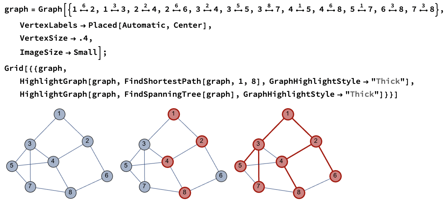
其中:
- 对于无向图中的符号 ●–●, 其为
\[UndirectedEdge], 输入方法为ESC ue ESC. 通过Ctrl - 7可以输入上标, 上标对应的是边的权值, 或者可以用 UndirectedEdge 来直接输入:UndirectedEdge[u, v, t]. - 使用 FindShortestPath 来找到图中最短的路径.
使用
Method参数可以指定找到最短路径的算法: Dijkstra, BellmanFord. (注: 其他还有 Floyd-Warshall 算法)适用于货物运输问题, 设备更新问题这样的有一个起点和终点的规划模型的问题. 一般的想法是首先建立节点和节点之间的权, 最后使用找最短路径的方式来解决问题.
- 使用 FindSpanningTree 来找到一个最小生成树. 可用的 Method 有:
Kruskal, Minimum cost arborescences, Prim.
适用于通信建设, 管道铺设规划, 这样的没有起点和终点的规划模型的问题. 即想要让所有的点连接在一起的最小连接方法的问题.
蚁群算法
在一个图中, 如何求得遍历所有点的最短路径的方法. 且只经过城市 1 次. 其思想从蚁群如何寻找最短路径而来:
- 蚂蚁经过路径会留下信息浓度 $τ$, 其与经过路径的长度 $d_{ij}$ 成反比.
- 蚂蚁在分叉路上更可能选择信息素浓度高的方向移动, 即
$$P_{ij}^k(t) = \left\{\begin{array}{ll}\frac{τ_{ij}(t)}{∑_{s ∈ allowed_k} τ_{is} (t)} & j ∈ allowed_k \\ 0 & j ∉ allowed_k \end{array}\right.$$
其中, $P_{ij}^k(t)$ 为在 $t$ 时刻第 $k$ 只蚂蚁选择从 $i$ 到 $j$ 的概率. $allowed_k$ 为 $k$ 蚂蚁未经过的城市集合.
为了加速收敛速度, 考虑距离的影响:
$$P_{ij}^k(t) = \left\{\begin{array}{ll}\frac{[τ_{ij}(t)]^α × [\frac{1}{d_{ij}(t)}]^β}{∑_{s ∈ allowed_k} [τ_{is} (t)]^α × [\frac{1}{d_{is}(t)}]^β} & j ∈ allowed_k \\ 0 & j ∉ allowed_k \end{array}\right.$$
- 若 $β = 0$, 则完全为正反馈算法, 收敛速度较慢
- 若 $α = 0$, 则完全为贪心算法, 容易陷入局部极值
- 信息素随时间挥发, 故 $i$ 和 $j$ 节点之间 $t$ 时刻的信息素记为 $τ_{ij}(t)$. 则 $τ_{ij}(t + 1) = (1 - ρ) τ_{ij} (t) + ∑_{k = 1}^m Δ τ_{ij}^k, 0 < ρ < 1$. 其中 $Δ τ_{ij}^k = \frac{Q}{L_k}$ 若 $k$ 经过 $d_{ij}$, 否则为 $0$, $L_k$ 为总路径长度; $ρ$ 为一个信息素消失的速度. $Q$ 为一个常数.
其他资源 (MMA):
神经网络
适用于: 预测类, 分类, 评价类型的问题.
感知机
一个感知机模型 (最简单的神经网络) 由如下的部分组成:
- 输入层: Input 为输入的信号 $x$
- 激活函数: 综合判断输入信号是否达到 阀值
- 输出层: Output 激活函数在输出层, 求得的函数就是输出值 $y$
示意图:

若要在上面的模型中加入一个阈值.

于是就可以加入一个阀值的考虑, 如果 f(x) = x < 0 ? 0 : 1,
那么就变成了一个决断系统了.
注: 如果用 Mathematica 来的话, 就变成了一个简单的 LinearLayer:
layer = LinearLayer[1, "Input" -> 3]
大概就是这个样子的.
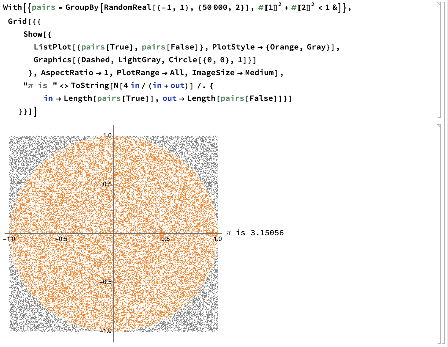
蒙特卡洛法
当无法求得精确解的时候, 通过随机抽样, 根据统计试验求近似解. 适用于可行域过大, 没有通用方法求出精确解的问题.
注: 为了满足统计意义, 需要抽样数足够多.
一个经典例子:
蒙特卡洛法可以配合用于非线性规划来计算初始值, 用于在非线性规划中辅助计算:
- 对于非线性多元函数 $f(\boldsymbol{x})$, 有 $n$ 个变元 $x_i$. 现在要在一组约束 $g_i(\boldsymbol{x})$ 下计算 $f$ 的最大 (小) 值.
- 随机生成 $n$ 个变元, 记为 $\boldsymbol{x}^{(k)}$.
- 判断约束 $g_i$ 是否被满足, 若是, 则进入下一步; 若否, 则重新生成.
- 判断该结果是否为更大 (小) 值, 若是, 则更新最大 (小) 值; 若否, 则回到生成步骤重新开始.
其他参考:
传播模型
可以参考 Compartmental models in epidemiology. 下面的模型原理非常简单, 基本只要搞清楚转换关系和约束关系即可.
指数传播模型
- $t$ 时刻传播数 $N(t)$
- 单位时间传播的数量 $λ N(t) Δ t$
- 方程: $N(t + Δ t) = N(t) + λ N(t) Δ t$, 结果为 $N = N_0 e^{λ t}$ 类型的指数传播模型.
- 一般只能用于描述初期的问题, 不太合理.
SI 模型
- 总数 $N$, 认为是不考虑变化的常数
- 将人群分为易感染 (susceptible, 可感染) 和已感染 (infective), 用占比 $s(t)$ 和 $i(t)$ 来表示, 有 $s(t) + i(t) = 1$. 忽略治愈和死亡.
- 感染率: 已感染者每天接触的平均人数 $λ$ (日感染率), 接触可感染者时, 会将其感染成病人, 故一个已感染者传播的人数即为其接触的可感染人数 $λ s(t)$.
- 方程: $N i(t + Δ t) - N i(t) = λ N s(t) i(t) Δ t$.
一个例子:
NDSolve[{i'[t] == 0.5* s[t] * i[t], s[t] + i[t] == 1, i[0] == 0.001},
  {s, i}, {t, 0, 30}];
Plot[Evaluate[{s[t], i[t]} /. %[[1]]], {t, 0, 30}, PlotRange -> All]
- 用 $i'(t)$ 来表示传染病曲线, 在高峰期 $i = 0.5$, 有 $t_m = \frac{1}{λ} \mathrm{ln} (\frac{1}{i_0} - 1)$
- 但是没有考虑治愈
SIS
- 在 SI 模型上考虑治愈比例 $μ$, 即每天被治愈的病人占总数的比例. 以及无免疫性, 即被治愈后仍然可以被感染.
- 于是新的方程为:
$$\left\{\begin{array}{llll} i'(t) & = & λ i(t) (1 - i(t) - μ i(t)) & t > 0\\i(0) & = & i_0 & \end{array}\right.$$
SIR
- 考虑治愈后不会被感染
- $s'(t) = - λ i(t) s(t)$ 可感染人数的变化, 即被感染后的人数每天可以接触 $λ$ 人.
- $i'(t) = λ i(t) s(t) - μ i(t)$ 感染人数的变化为被感染的减去治愈的
- $r'(t) = μ i(t)$ 感染后治愈的人数的变化
- $i(t) + s(t) + r(t) = 1$ 为总人数
马尔科夫链
适用于状态随机, 下一阶段只和当前状态有关的问题, 如健康变化, 销售储存, 等价结构变化这样的问题.
其他的参考资料:
一个题外话
后悔, 总之现在就是非常后悔, 如果当时我在概统课上好好听老师讲的关于赌博的问题的话, 现在估计也不会花这么多的时间来学这些了. 害.