Brief Surf of Computational Physics
About
这是用于计算物理模拟考试的一个快速复习的东西.
不过需要注意的是, 本文会用 Lisp (或者有可能有别的吧) 作为算法, 以及代码的例子. 不过是出于个人的 XP 和熟练程度做出的考量罢了.
如果你对 CL (Common Lisp) 比较好奇的话, 可以参考文末的 Appendix 介绍. 或者倒不如说, 如果对 CL 比较陌生的话, 可以参考文末的 Appendix 的介绍.
虽然不是很想说 Python 调包真的是很爽, 也不想吹嘘 Lisp 直接写也很不错. 不过在论坛 (kernel) 上我有随着上课做同步的一个 (主要为) Python 的一个 writeUP.
所有的代码都将放在 computational-physics.lisp 中:
(defpackage #:computational-physics
  (:use :cl :gurafu)
  (:nicknames :phy))

(in-package :phy)
(不过在我写完之后感觉这些代码写得并不怎么样, 总觉得还是不够优雅)
Overview

Numbers and Precision
数制的表示
- \(p\) 进制整型:
(defun p-base-integer (p bits)
  "Trun a list of `p' base bits into integer.
Return an integer crossponding to `bits'.

  (a_n a_{n-1} ... a_1 a_0) = sum a_i p^i

For example:

  (p-base-integer '(0 0 1 1) 2) => 3
"
  (flet ((scanner (int bit)
           (assert (< -1 bit p))
           (+ (* p int) bit)))
    (reduce #'scanner bits :initial-value 0)))

(defun integer-p-base (p integer &optional bits)
  "Trun `interger' to a list of `p' base bits.
Return a list of `p' base bits.
"
  (if (zerop integer) bits
      (integer-p-base p (floor integer p) (cons (mod integer p) bits))))
- \(p\) 进制小数:
(defun p-base-decimal (p bits)
  "Trun a list of `p' base decimal bits into a decimal number.
Return a float number crossponding to `bits' [0, 1).

  (b_1 b_2 ... b_n) = sum b_i p^{-i}

For example:

  (p-base-decimal '(1) 4) => 0.25
"
  (flet ((scanner (int bit) (+ (float (/ int p)) bit)))
    (float
     (/ (reduce #'scanner (reverse bits) :initial-value 0) p))))

(defun decimal-p-base (p decimal &optional bits)
  "Trun a decimal to `p' base bits.
Return a p base bits list.
"
  (if (zerop decimal) bits
      (let ((shifted (* p decimal)))
        (decimal-p-base p (mod shifted 1.0)
                        (cons (truncate (mod shifted p)) bits)))))
这里有一个小小的坑, 其实浮点数在计算机中的表示是有极限的, 并不能准确地描述任意精度的浮点数:
;; single float
(type-of 0.1)            ;; => single-float
(decimal-p-base 2 0.1)   ;; => (1 0 1 1 0 0 1 1 0 0 1 1 0 0 1 1 0 0 1 1 0 0 1 1 0 0 0)

;; double float
(type-of 0.1d0)          ;; => double-float
(decimal-p-base 2 0.1d0) ;; => (1 0 1 1 0 0 1 1 0 0 1 1 0 0 1 1 0 0 1 1 0 0 1 1 0 0 1 1 0 0 1 1 0 0 1 1 0 0 1 1 0 0 1 1 0 0 1 1 0 0 1 1 0 0 0)
- \(p\) 进制实数
(defun p-base-real (p int-bits dec-bits)
  "Return a `p' base real number for `int-bits' and `dec-bits'.

  real = integer + decimal
"
  (+ (p-base-integer p int-bits)
     (p-base-decimal p dec-bits)))
Reader Macro
(这部分的代码将会被省略)
(defun p-real-reader (stream subchar arg)
  "Read a p base number like `#p2:01010.01010'. "
  (declare (ignore subchar arg))
  (flet ((check (bit p)
           (if (< bit p)
               bit
               (error (format nil "~d is not ~d-base bit." bit p))))
         (read-bit ()
           (let ((char (read-char stream nil #\ )))
             (cond ((char<= #\0 char #\9)
                    (- (char-code char) (char-code #\0)))
                   ((char<= #\A char #\Z)
                    (+ 10 (- (char-code char) (char-code #\A))))
                   ((char<= #\a char #\z)
                    (+ 10 (- (char-code char) (char-code #\a))))
                   ((or (char= char #\:) (char= char #\.)) -1)
                   (t (unread-char char stream) -1)))))
    (let ((p 0) int dec)
      ;; read p
      (loop for bit = (read-bit)
            while (>= bit 0)
              do (setf p (+ (check bit 10) (* 10 p))))

      ;; read int
      (loop for bit = (read-bit)
            while (>= bit 0)
              do (push (check bit p) int))

      ;; read dec
      (loop for bit = (read-bit)
            while (>= bit 0)
              do (push (check bit p) dec))

      ;; return p-base-real
      (p-base-real p (nreverse int) (nreverse dec)))))

(set-dispatch-macro-character #\# #\p #'p-real-reader)
于是对于 Lisp, 你可以这样表示一个数:
#p10:23.333, 或者是#p2:1010.1(10.5). - IEEE 浮点数
将一段二进制空间划分为三个部分:
sign,exponent,fraction, 每部分视为一段 2 进制数, 然后按照规则将其拼接在一起:\[(-1)^{\mathrm{sign}} × 2^{\mathrm{exponent} - \mathrm{offset}} × (1 . \mathrm{fraction})\]
其中
offset为exponent的长度, 对于几个特殊的情况:Exponent fraction = 0 fraction != 0 Note 0 0 subnormal number (见 wikepedia) offset = offset - 1 max infinity NaN offset = offset else normal normal 一般的做法变成:
(defun from-ieee-float (sign exponent fraction
                        &optional
                          (offset (1- (expt 2 (1- (length exponent)))))
                          (max-exponent (1- (expt 2 (length exponent)))))
  "Trun a IEEE float to float. "
  (let* ((sign     (if (zerop sign) 1 -1))
         (exponent (p-base-integer 2 exponent))
         (fraction (p-base-decimal 2 fraction))
         (type (cond ((= exponent max-exponent)
                      (if (zerop fraction)
                          (if (> sign 0)
                              :positive-infinity
                              :negative-infinity)
                          :nan))
                     ((zerop exponent)
                      (if (zerop fraction) :zero :subnormal))
                     (t :normal))))
    (values (if (eq type :normal)
                (float (* sign (expt 2 (- exponent offset)) (1+ fraction)))
                (float (* sign (expt 2 (- 1 offset)) fraction)))
            type)))
- IEEE 754 (32 位浮点数)
offset = 127,max-exponent = 255(defun ieee-float (bits) "Return float from IEEE 754 float `bits'. HIGH LOW sign exponent fraction 0 1 9 32 " (let ((sign (first bits)) (exponent (subseq bits 1 9)) (fraction (subseq bits 9 32))) (from-ieee-float sign exponent fraction 127 255)))
- IEEE 754 half (16 位浮点数)
offset = 15,max-exponent = 31(defun ieee-half-float (bits) "Return IEEE 754 half float from `bit' HIGH LOW sign exponent fraction 0 1 6 16 " (let ((sign (first bits)) (exponent (subseq bits 1 6)) (fraction (subseq bits 6 16))) (from-ieee-float sign exponent fraction 15 31)))
- Reader Macro
实现略
(这部分的代码也应当被忽略)
(defun ieee-float-reader (stream subchar arg)
  "Read a IEEE float like `#f0011110000000000' for half float,
and `#F11000000000000000000000000000000' for float. "
  (declare (ignore arg))
  (flet ((read-n-bits (n)
           (loop repeat n
                 for bit = (let ((char (read-char stream)))
                             (cond ((char= char #\0) 0)
                                   ((char= char #\1) 1)
                                   (t (unread-char char stream) nil)))
                 while bit
                 collect bit)))
    (cond ((char= subchar #\f) (ieee-half-float (read-n-bits 16)))
          ((char= subchar #\F) (ieee-half-float (read-n-bits 32)))
          (t (error "Unsupported. ")))))

(set-dispatch-macro-character #\# #\f #'ieee-float-reader)
(set-dispatch-macro-character #\# #\F #'ieee-float-reader)
于是就可以如下表示浮点数:
#F11000000000000000000000000000000, 或者#f0011110000000000. - 编码
- IEEE 754 (32 位浮点数)
精度
通过泰勒展开消除小量带来的误差 Catastrophic Cancellation
对于表达式 \(f(x)\) 在 \(x → 0\) 的时候, 直接计算可能会有精度上的损失, 可以通过小量展开将函数化简来解决:
\[f(x) = f(x_0) + (x - x_0) \frac{\mathrm{d} f(x_0)}{\mathrm{d} x} + o\left( (x - x_0)^2 \right)\]
- 对于 \(N → ∞ ⇒ N = \frac{1}{x}, x → 0\), 通过变量变换进行替换计算.
- 对于积分的表达式的计算: \(∫_N^{N + 1} f(x) \mathrm{d} x = F(N + 1) - F(N) = ∂_N F(N) = f(N)\).
Condition Number
Condition Number 描述了一个函数相对输入的变化情况.
\[κ(f, x) = lim_{ε → 0} \mathrm{sup}_{\left\Vert δ x \right\Vert \leq ε} \frac{\left\Vert δ f(x) \right\Vert}{\left\Vert f(x) \right\Vert} / \frac{\left\Vert δ x \right\Vert}{\left\Vert x \right\Vert}\]
对于一元函数:
\[κ(f, x) = \left| \frac{x f'(x)}{f(x)} \right|\]
对于多元函数:
\[κ(f, x) = \left| \frac{\left\Vert \boldsymbol{J}(x) \right\Vert}{\left\Vert f(x) \right\Vert / \left\Vert \boldsymbol{x} \right\Vert} \right|\]
这里可以给一个实验的角度
- 测量时的误差 \(σ\), 相对误差 \(\frac{σ}{f}\)
- Condition Number \(κ\) 表示了入参的误差对于函数值的影响程度
- 在误差传递的过程中 \(σ_f = \sqrt{(∂_{x_i} f)^2 σ_{x_i}^2}\) (误差传递公式)
- 于是可以得到 \(\frac{σ_f}{f} = \sqrt{(∂_{x_i} f)^2 σ_{x_i}^2 / f^2} = κ \frac{σ_a}{a}\) \(⇒ κ = \sqrt{a^2 (∂_{x_i} f)^2 σ_{x_i}^2 / f^2 σ_a^2}\).
Richardson Extrapolation
在计算导数的时候, 很容易陷入 \(f(x + δ x) - f(x)\) 这样的因为小量误差导致的 \(f(x + δ x) - f(x) → 0\).
解决方法就是使用 Richardson Extrapolation 对函数进行展开:
\[\begin{matrix} A(h) = f(x + h) - f(x) + O(h) \ A(h) = B(h) + o(h^{k+1}) \ B(h) = \frac{2^k A(\frac{h}{2}) - A(h)}{2^k - 1} \end{matrix}\]
(defun richardson-extrapolation (fn &optional (k 1))
  "Apply `k' rank Richardson Extrapolation on function `fn'. "
  (declare (type (integer 0) k))
  (if (zerop k) fn
      (let ((2expk (ash 2 k)))
        (lambda (h)
          (/ (- (* 2expk (funcall fn (/ h 2.0d0))) (funcall fn h))
             (1- 2expk))))))
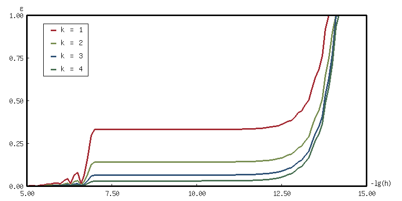
这里是一个例子: \(cos x = ∂_x sin x = \frac{sin (x + h) - sin x}{h}\)
(with-present-to-file
    (plot plot :margin 10
               :x-label "-lg(h)" :y-label "ε"
               :x-min 5 :x-max 15
               :y-min 0.0 :y-max 1.0)
    (out-path  :width 800)
  (flet ((data (k)
           (let* ((fn (lambda (h) (/ (- (sin (+ x h)) (sin x)) h)))
                  (rk  (richardson-extrapolation fn k))
                  (cos (cos x)))
             (loop for x from 5 below 15 by 0.1
                   for h = (expt 10 (- x))
                   collect (list x (abs (- (funcall rk h) cos)))))))
    (add-plot-data plot (line-plot-pane rk1 :color +大红+) (data 1))
    (add-plot-data plot (line-plot-pane rk2 :color +鹅黄+) (data 2))
    (add-plot-data plot (line-plot-pane rk3 :color +天蓝+) (data 3))
    (add-plot-data plot (line-plot-pane rk4 :color +豆绿+) (data 4))
    (add-plot-legend (plot)
      ("k = 1" :color +大红+)
      ("k = 2" :color +鹅黄+)
      ("k = 3" :color +天蓝+)
      ("k = 4" :color +豆绿+))))
out-path
随机数
随机数算法
LCG
\[s_{k+1} = (a × s_k + b)\ \mathrm{mod}\ m\]
随机数测试
Uniform
Percolation
Cluster
Numeric Calculus
Taylor Series
基本上可以看作是数值分析的基础了(?)
\[f(x + h) = ∑ \frac{h^n}{n!} f^{(n)}(x)\]
Numeric Differentiation
考虑对 \(\left\{ f(x + h_i) \right\}\) 展开到 \(n\) 阶可以得到的方程组, 变元为 \(f^{(i)}(x)\):
\[\left\{ ∑ \frac{h^i}{i!} f^{(i)}(x) = f(x + h_i) - f(x) \right\}\]
这里将其写作:
\[\boldsymbol{H} \left\{ f^{(i)}(x) \right\} = \left\{ f(x + h_i) - f(x) \right\}\]
通过构造逆矩阵 \(\boldsymbol{H}^{-1}\) 即可计算 \(f^{(i)}(x)\) 的表达式 (值).
构造系数矩阵以及求解表达式
这里通过 LLA 来进行矩阵的求解之类的问题, 不过之后估计可以自己写一个替换.
(defun make-hs-matrix (hs)
  "Make H matrix for hs.
Return a n*n array (matrix).

  H { f^{(i)}(x) } = { f(x + h_i) - f(x) }
"
  (let ((n (length hs)))
    (flet ((hw (h)
             (loop for i below n
                   for hi = h then (* hi h)
                   for i! = 1 then (* i! i)
                   collect (float (/ hi i!)))))
      (make-array (list n n) :initial-contents (mapcar #'hw hs)))))

(defun make-fs-matrix (n)
  "Make a F matrix for `n' f(x + h_i).
Return a (n+1)*n matrix.

  F { f(x), f(x + h_i) } = { f(x + h_i) - f(x) }
"
  (let ((f-mat (make-array (list n (1+ n)) :initial-element 0)))
    (loop for j below n do
      (setf (aref f-mat j (1+ j)) 1     ; f_{i+1,j} = 1
            (aref f-mat j 0)      -1))  ; f_{0,j}   = -1
    f-mat))

(defun make-finite-differentor-matrix (hs)
  "Make a matrix for finite differentor calculation.

  M = H^{-1} F; M { f(x), f(x + h_i) } = { f^{(i)}(x) }
"
  (let* ((n (length hs))
         (mat-h (make-hs-matrix hs))
         (mat-f (make-fs-matrix n)))
    (lla:mm (lla:invert mat-h) mat-f)))
可以来计算一下几个不同的微分算子的 \(\boldsymbol{M}\):
- first forward
(make-finite-differentor-matrix '(1))
#2A((-1.0d0 1.0d0)) - first backward
(make-finite-differentor-matrix '(-1))
#2A((1.0d0 -1.0d0)) - first centeral
(make-finite-differentor-matrix '(1 -1))
#2A((0.0d0 0.5d0 -0.5d0) (-1.0d0 0.5d0 0.5d0)) - \(f(x + \left\{ h, 0, 2 h \right\})\)
(make-finite-differentor-matrix '(1 2))
#2A((-1.5d0 2.0d0 -0.5d0) (0.5d0 -1.0d0 0.5d0))Note: 理论解为 \(2 f(x + h) - \frac{3}{2} f(x) - \frac{1}{2} f(x + h)\)
- \(f(x + \left\{ -2h, -h, h, 2h \right\})\)
(make-finite-differentor-matrix '(-2 -1 1 2))
#2A((-2.9802322387695313d-8 0.08333337306976318d0 -0.6666666865348816d0
     0.6666666865348816d0 -0.0833333432674408d0)
    (-1.2499999403953552d0 -0.041666656732559204d0 0.6666666269302368d0
     0.6666666269302368d0 -0.041666656732559204d0)
    (0.0d0 -0.1666666716337204d0 0.3333333432674408d0 -0.3333333432674408d0
     0.1666666716337204d0)
    (1.4999998658895493d0 0.24999994039535522d0 -0.9999998807907104d0
     -0.9999998807907104d0 0.24999995529651642d0))
Note: 理论值为 \(\frac{1}{12} f(x - 2h) - \frac{2}{3} f(x - h) + \frac{2}{3} f(x + h) - \frac{1}{12} f(x + 2h)\), (
1/12 = 0.0833,2/3 = 0.6666).不过这里也看出因为求逆矩阵过程中累计了误差, 导致后面计算的精度就会掉下去了. 不过暂时没有很好的解决方法, 先采用鸵鸟战术.
(defun make-finite-differentor (hs &optional (dx 1e-3) (d 1))
  "Make a finite differentor with `hs'. "
  (let ((rank (1- d)))
    (lambda (fn &optional (dx dx))
      (let* ((hs (mapcar (lambda (h) (* h dx)) hs))
             (mat (make-finite-differentor-matrix hs))
             (hs* (cons 0 hs)))
        (lambda (x)
          (flet ((f (h) (funcall fn (+ x h))))
            (aref (lla:mm mat (map 'vector #'f hs*)) rank)))))))

(defmacro finite-diff ((&rest hs) &key (dx 1e-3) (d 1))
  "Wrapper for `make-finite-differentor'. "
  `(make-finite-differentor (list ,@hs) ,dx ,d))
注: 这里主要因为最近在看 SDF 对 Scheme 类型的直接定义 Lambda 的方式比较欣赏.
不过代价就是在 Common Lisp 里面调用需要用 funcall 而不能直接用结果.
可能会有更加好用的方式, 暂时不清楚.
于是对于不同的微分算子, 都可以通过这样的方式来进行离散化:
这里用一些比较简单的例子来对结果进行简单的验证:
- first forward: 通过 \(f(x), f(x + h)\) 作为采样点来计算导数
(defparameter first-forward (finite-diff (1))
  "First forward different.

  f'(x) = (f(x + h) - f(x)) / h")
(defparameter first-backward (finite-diff (-1))
  "First backward different.

  f'(x) = (f(x) - f(x - h)) / h")
(defparameter first-central (finite-diff (-1 1))
  "First central different.

  f'(x) = (f(x + h) - f(x - h)) / (2 * h)")
这里会同样遇到前文的精度的问题, 比如构造一个误差的记录函数:
(defun 2-fn-rms-error (f1 f2 xmin xmax &optional (dx 0.1))
  (flet ((square (x) (* x x)))
    (loop for x from xmin to xmax by dx
          collect (square (- (funcall f1 x) (funcall f2 x))) into sum
          finally (return (sqrt (reduce #'+ sum))))))
| dx | rms-error |
| 1/10 | 0.19810856549617295d0 |
| 1/100 | 0.01981925960583512d0 |
| 1/1000 | 0.0019056572355073285d0 |
| 1/10000 | 0.0030402329579347367d0 |
| 1/100000 | 0.012121302612617568d0 |
| 1/1000000 | 0.18903780629484798d0 |
就会发现一开始随着 dx 的减小, 精度会提升, 但是随着 dx 的进一步减小,
精度会因为计算误差而下降, 解决方法有两种:
- 通过 Richardson Extrapolation 进行展开
\[A = A(h) + K h^k + O(h^{k+1})\] \[A = B(h) + O(h^{k+1})\] \[B(h) = \frac{2^k A(\frac{h}{2}) - A(h)}{2^k - 1}\]
略
make-finite-differentor的修改:(defun calculate-differential (fn x hs) "Calculate { f^{(i)}(x + hs_i) } with function `fn' at `x'. " (let* ((mat (make-finite-differentor-matrix hs)) (hs* (cons 0 hs))) (lla:mm mat (map 'vector (lambda (h) (funcall fn (+ x h))) hs*)))) (defun make-finite-differentor* (hs &optional (dx 1e-3) (richard-k 1) (d 1)) "Make a finite differentor with `hs' using Richard Extrapolation. " (let ((rank (1- d))) (lambda (fn &optional (dx dx)) (lambda (x) (let* ((df (lambda (h) (aref (calculate-differential fn x (mapcar (lambda (hi) (* h hi)) hs)) rank))) (rk (richardson-extrapolation df richard-k))) (funcall rk dx))))))
- 一个简单的测试:
绘图代码折叠了
(with-present-to-file
    (plot plot :margin 10
               :x-label "-lg(dx)" :y-label "ε"
               :x-min 1   :x-max 10
               :y-min 0.0 :y-max 5)
    (out-path  :width 800)
  (loop with hs = '(1)
        for n from 1 to 10 by 0.1
        for dx = (expt 10 (- n))
        collect
        (let ((d-rk0 (make-finite-differentor  hs dx))
              (d-rk1 (make-finite-differentor* hs dx 1))
              (d-rk2 (make-finite-differentor* hs dx 2))
              (d-rk3 (make-finite-differentor* hs dx 3)))
          (mapcar (lambda (d)
                    (list n (2-fn-rms-error (funcall d #'sin) #'cos 0 pi)))
                  (list d-rk0 d-rk1 d-rk2 d-rk3)))
          into data-trans
        finally
           (destructuring-bind (rk0 rk1 rk2 rk3)
               (print (apply #'mapcar #'list data-trans))
             (add-plot-data plot (line-plot-pane rk0 :color +大红+) rk0)
             (add-plot-data plot (line-plot-pane rk1 :color +鹅黄+) rk1)
             (add-plot-data plot (line-plot-pane rk2 :color +天蓝+) rk2)
             (add-plot-data plot (line-plot-pane rk3 :color +豆绿+) rk3)
             (add-plot-legend (plot)
               ("k = 0" :color +大红+)
               ("k = 1" :color +鹅黄+)
               ("k = 2" :color +天蓝+)
               ("k = 3" :color +豆绿+)))))
out-path
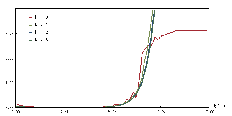
又是看图说话的时候了… 这让我有些惊讶, 实际上一开始以为
dx应该是越小越好, 毕竟切线是割线的极限嘛 (诶, 学数学学的), 实际上是在 0.001 附近倒是最好的; 并且还认为 Richard Extrapolation 的效果一定会比默认的要好, 结果发现其实不然 (我这里把图的 Y 轴拉得很大, 结果会发现, 都是出现非常扯淡的结果, 但是朴素的算法竟然意外的能打,虽然都差得很多就是了. ) - 另一个测试:
绘图代码还是折叠了
(with-present-to-file
    (plot plot :margin 10
               :x-label "-lg(dx)" :y-label "ε"
               :x-min 1   :x-max 6
               :y-min 0.0 :y-max 0.05)
    (out-path  :width 800)
  (macrolet ((:> (hs rk0 rk1 rk0-color rk1-color)
               `(loop with hs = ',hs
                      for n from 1 to 6 by 0.1
                      for dx = (expt 10 (- n))
                      collect
                      (let ((d-rk0 (make-finite-differentor  hs dx))
                            (d-rk1 (make-finite-differentor* hs dx 1)))
                        (mapcar (lambda (d)
                                  (list n (2-fn-rms-error (funcall d #'sin)
                                                          #'cos 0 pi)))
                                (list d-rk0 d-rk1)))
                        into data-trans
                      finally
                         (destructuring-bind (rk0 rk1)
                             (print (apply #'mapcar #'list data-trans))
                           (add-plot-data plot
                             (line-plot-pane ,rk0 :color ,rk0-color) rk0)
                           (add-plot-data plot
                             (line-plot-pane ,rk1 :color ,rk1-color) rk1)))))
    (:> (1)    rk0 rk1 +大红+ +鹅黄+)
    (:> (1 -1) rk2 rk3 +天蓝+ +豆绿+))
  (add-plot-legend (plot :padding 0.1)
    ("k = 0 first forward"  :color +大红+)
    ("k = 1 first forward"  :color +鹅黄+)
    ("k = 0 first centeral" :color +天蓝+)
    ("k = 1 first centeral" :color +豆绿+)))
out-path
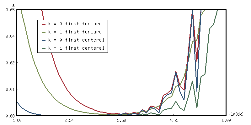
如此可见: 调
dx的作用可能比换算法来得有效, 并且与其纠结小量展开的误差, 其实考虑换一个求导方法估计效果更好.
- 通过使用虚数进行计算
\[f(x + i h) = f(x) + i h f'(x) + \cdots ⇒ f'(x) = \frac{\mathrm{Im}(f(x + i h))}{h} + \frac{h^2}{6} f”'(x) + O(h^4)\]
Numerical Integration
Taylor Expand
对于 \((a, b)\) 段上的积分 \(∫_a^b f(x) \mathrm{d} x\), 可以将其分成小份, 再通过 Taylor 展开转换为幂级数的积分:
\[∫_{a}^{b} f(x) \mathrm{d}x = ∑_{n = 0}^{∞} ∫_{x_0 - h}^{x_0 + h} \frac{x^i}{i!} f^{(i)}(x_0) \mathrm{d} x = ∑_{n = 0}^{∞} \frac{f^{2n} (x_0)}{(2n + 1)!} 2 h^{n + 1}\]
考虑其中的 \(∫_{-h}^{h}\) 的小份的积分:
(defun integrate (fn xmin xmax method &optional (dx 1e-3))
  "Integrate function `fn' from `xmin' to `xmax' with `method'. "
  (loop with integrate = 0
        for x from xmin upto xmax by dx
        do (incf integrate (funcall method fn x dx))
        finally (return integrate)))
- Midpoint Rule: \(2 h f(\frac{a + b}{2}) + o(h^{3})\) 对应一阶的展开
Midpoint Rule
(defun midpoint-rule (fn x 2h)
  "Integarate function `fn' from `xmin' to `xmax'. "
  (* 2h (funcall fn (+ x (/ 2h 2)))))
- Simpson Rule: \(2 h f(x_0) + \frac{f”(x_0)}{3} h^3 + o(h^5)\) 对应二阶的展开
其中使用符号求导的结果替换 \(f”\) 项 (利用前文的
(make-finite-differentor-matrix '(1 -1))):\[∫_a^b f(x) \mathrm{d}x = \frac{h}{3} \left[ f(a) + 4 f(\frac{a + b}{2}) + f(b) \right]\]
Simpson Rule
(defun simpson-rule (fn x 2h)
  "Integrate function `fn' from `xmin' to `xmax'. "
  (* 2h 1/2 1/3
     (+ (funcall fn x)
        (* 4 (funcall fn (+ x (/ 2h 2))))
        (funcall fn (+ x 2h)))))
- 同样的, 和导数一样, 有虚数形式:
\[∫_a^b f(x) \mathrm{d}x = \left[ ∑_{i=0}^{n-1} 2 h f(a + i h) \right] + o(h^2)\]
考虑误差的累积
(with-present-to-file
    (plot plot :margin 10
               :x-label "ln(dx)" :y-label "ln(ε)"
               :x-min 1d-6   :x-max 1d-1
               :y-min 1d-14  :y-max 1d-1
               :scale :log-log)
    (out-path  :width 800)
  (flet ((fn (x) (* x (exp x)))) ;; => F(x) = (x - 1) * e^x => integrate = 1
    (flet ((data (method)
             (loop for n from 1d0 to 6d0 by 0.1d0
                   for dx = (expt 10d0 (- n))
                   collect (list dx (abs (1- (integrate #'fn 0 1 method dx)))))))
      (add-plot-data plot (line-plot-pane midpoint :color +大红+)
        (data #'midpoint-rule))
      (add-plot-data plot (line-plot-pane simpson  :color +天蓝+)
        (data #'simpson-rule))))
  (add-plot-legend (plot :padding 0.0)
    ("Midpoint Rule" :color +大红+)
    ("Simpson Rule"  :color +天蓝+)))
out-path
emmm… 两个之间的误差基本可以忽略了. 直接计算的话, Simpson Rule
(integrate #'sin 0 pi #'simpson-rule) 结果为 2.0000064;
Midpoint Rule (integrate #'sin 0 pi #'midpoint-rule) 的结果为 2.0000067.
可能还跟浮点数精度有关. 用双精度的话, (integrate #'sin 0 pi #'simpson-rule 1d-3)
的结果为 1.9999999170346228d0; (integrate #'sin 0 pi #'midpoint-rule 1d-3) 的结果为
2.0000000003679577d0.
Newton-Cotes Weights
不难发现, 上面的 Taylor Expand 是假设采样点都是均匀分布的 (确切来说, 是二等分的). 那如果对于非等分, 或者说任意的采样点呢? 即:
\[∫_a^b f(x) \mathrm{d} x = ∑_i w_i f(x_i), x_i ∈ [a, b]\]
因为 \(w_i\) 因与 \(f(x)\) 无关, 所以可以代入 \(f(x) = 1, x, x^2\), 于是问题又变成了求解线性方程组.
- Rectangle Rule: \(∫_{x_1}^{x_2} f(x) \mathrm{d}x = h f_1\)
- Trapezium Rule: \(∫_{x_1}^{x_2} f(x) \mathrm{d}x = \frac{h}{2} (f_1 + f_2) + o(h^3)\)
(其实这部分完全就是矩形规则和梯形规则嘛… )
Romberg's Method
如何消除小量的误差? 还是 Richardson Extrapolation.
Gaussian Quadrature
\[∫_{-1}^1 f(x) \mathrm{d} x = f(\frac{1}{\sqrt{3}}) + f(- \frac{1}{\sqrt{3}})\]
Symbolic Differentiation
这部分可以参考: What about Symbolic df?, 这里就不写了, 因为不是重点. 不过我现在对之前的代码又有些不太满意了, 底层写得太死了, 无法支持更加灵活的修改. 拓展性不足.
Solving Equations
(注: 复习时间不太多了, 一些不常用的我就跳过了… 这里建议后面的参考 kernel 上的笔记)
One Variable
方程的求解方式即构造一个迭代器, 以及提供一个更新方法, 若更新的解不够好, 就继续更新, 反之则返回更新的解:
(defun convergence (update-fn init-x
                  &key (tol 1e-3)
                    (diff (lambda (a b) (abs (- a b)))))
  "Calculate the root with `update-fn' with `init-x'. "
  (labels ((iter (x)
             (let ((update-x (funcall update-fn x)))
               (if (< (funcall diff x update-x) tol) update-x
                   (iter update-x)))))
    (iter init-x)))
对于类似这样的迭代法的通用思路, 有一套专门描述的理论语言:
- Q-convergence: 在迭代的过程中, 每次更新的量 \(| x_{k+1} - x_k | = | ε_k |\) 有:
\[lim_{k → ∞} \frac{| ε_{k+1} |}{| ε_k |^q} = μ\]
如何计算这个
很遗憾, 只能理论推导 (手算) 吗?- 令 \(x_{k+1} = φ(x_k), ξ = lim_{k → ∞} φ(x_k)\)
- \(ε_{k+1} = ε_k φ'(ξ) ⇒ lim_{k → ∞} \frac{| ε_{k+1} |}{| ε_k |^q} = μ\)
- \(μ\) 表示了收敛的速度
- \(q\) 表示了收敛的阶数 (order)
- 近似值: (可以通过在迭代时候计算)
\[q ≈ \frac{log \left| \frac{x_{k+1} - x_k}{x_k - x_{k-1}} \right|}{log \left| \frac{x_k - x_{k-1}}{x_{k-1} - x_{k-2}} \right|}\]
- 可收敛区域 (并不是所有初始点都可以收敛的)
Rearrange 不动点求解
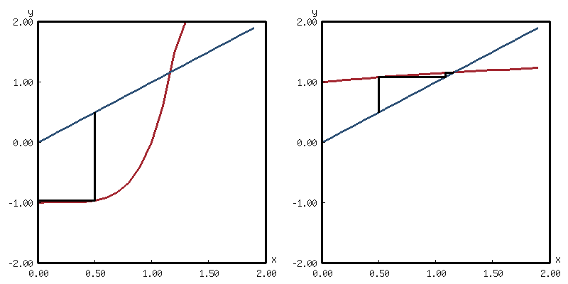
对于方程 \(\mathrm{eq}(x) = 0\), 手动变换形式为 \(x = f(x)\), 可以发现变成了一个求解不动点的问题. 于是迭代就可以计算得到最后的结果.
一个例子
对于: \(x^5 - x - 1 = 0 ⇒ x = (x + 1)^{1/5}\), 可以计算得到:
(convergence (lambda (x) (expt (1+ x) 1/5)) 1) ;; => 1.1672806
为什么不用 \(x = x^5 - 1\)?
emmm… 这里是一个简单的图示:
(with-present-to-file
    (plots horizontal-layout-presentation)
    (out-path :width 800)
  (flet ((data (fn) (loop for x from xmin upto xmax by 0.1
                          collect (list x (funcall fn x))))
         (draw-path (fn)
           (loop for i below 3
                 for x = 0.5 then y
                 for y = (funcall fn x)
                 collect (list x x)
                 collect (list x y))))
    (add-component plots 'a
                   (with-present (plot plot :margin 10
                                            :x-min xmin :x-max xmax
                                            :y-min ymin :y-max ymax)
                     (add-plot-data plot (line-plot-pane update :color +大红+)
                       (data (lambda (x) (1- (expt x 5)))))
                     (add-plot-data plot (line-plot-pane y=x :color +天蓝+)
                       (data #'identity))
                     (add-plot-data plot (line-plot-pane path)
                       (draw-path (lambda (x) (1- (expt x 5))))))
                   0.5)
    (add-component plots 'b
                   (with-present (plot plot :margin 10
                                            :x-min xmin :x-max xmax
                                            :y-min ymin :y-max ymax)
                     (add-plot-data plot (line-plot-pane update :color +大红+)
                       (data (lambda (x) (expt (1+ x) 1/5))))
                     (add-plot-data plot (line-plot-pane y=x :color +天蓝+)
                       (data #'identity))
                     (add-plot-data plot (line-plot-pane path)
                       (draw-path (lambda (x) (expt (1+ x) 1/5)))))
                   0.5)))
out-path
从图中不难看出收敛的迭代线 (黑色) 的变化趋势吧.
Newton Raphson Method
\[x_{k+1} = x_k - \frac{f(x_k)}{f'(x_k)}\]
(defun newton-raphson-solve (fn dfn init-x
                             &key (tol 1e-3)
                               (diff (lambda (a b) (abs (- a b)))))
  "Newton Raphson. "
  (convergence (lambda (x) (- x (/ (funcall fn x) (funcall dfn x))))
               init-x :tol tol :diff diff))
- \(q = 2\)
- \(μ = \frac{1}{2} \frac{f”(ξ)}{f'(ξ)}\)
Secant Method
当 Newton Raphson 在使用 first-forward 数值求导的时候, 就会变成 Secant Method:
\[x_{k+1} = x_k - f(x_k)\frac{x_k - x_{k-1}}{f(x_1) - f(x_0)}\]
- \(q = \frac{1 + \sqrt{5}}{2}\)
Bisection
\[a_{k+1}, b_{k+1} = φ(a_k, b_k) = \left\{ \begin{matrix} (a_k, \frac{a_k + b_k}{2}) & f(\frac{a_k + b_k}{2}) > 0 \ (\frac{a_k + b_k}{2}, b_k) & f(\frac{a_k + b_k}{2}) < 0 \end{matrix} \right.\]
- \(q = 1\)
- \(μ = \frac{1}{2}\)
注: 通过拓展是可以变成多维的形式的, 见后文.
Inverse Quadratic Interpolation
\[x_{n+1} = \frac{f_{n-1} f_n}{(f_{n-2} - f_{n-1}) (f_{n-2} - f_n)} x_{n-2} + \frac{f_{n-2} f_n}{(f_{n-1} - f_{n-2}) (f_{n-1} - f_n)} x_{n-1} + \frac{f_{n-2} f_{n-1}}{(f_n - f_{n-2}) (f_n - f_{n-1})} x_n\]
Multiple Variable
Optimize
Local
解方程 \(f'(x) = 0\)
把问题变成求解 \(f'(x) = 0\) 的解方程问题.
Gradient Descent
\[\boldsymbol{x}_{k+1} = \boldsymbol{x}_k + Δ \boldsymbol{x}_k = \boldsymbol{x}_{k+1} - α \frac{∇ f(\boldsymbol{x}_k)}{| ∇ f(\boldsymbol{x}_k) |}\]
其中缩放的尺度 \(α\) 通过 line search 方法进行确定:
- \(f(\boldsymbol{x}_{k+1}) - f(\boldsymbol{x}_k) < α c | ∇ f(\boldsymbol{x}_k) |\)
- 其中 \(c\) 为控制常数, \(α\) 通过 \(τ\) 进行缩放
(defmacro that (var &key condition improve initial)
  "Get the `var' that make the `condition' for true.
Improve the `var' using improve procedure. "
  `(loop for ,var = ,initial then ,improve
         while (not ,condition)
         finally (return var)))

;; pesudo-code
(that alpha
      :condition (let ((gradient (∇ f xk))
                       (xk+1 (- xk (* alpha (uniform gradient)))))
                   (< (- (f xk+1) (f xk)) (* -1 alpha c (norm gradient))))
      :improve (* alpha c)
      :initial 1)
(没时间了, 只能写伪代码了… )
Eigenvector Following
如果想要保证能够找到的就是最小值 (在一维问题的情况下, 这个可以通过 Newton Raphson 计算 \(x_{k+1} = x_k - \frac{f'(x)}{| f”(x) |}\) 来实现).
对于 Gradient Search, 这是将上文中的 ∇ 算子替换为在本征矢上的投影:
\[∇_{\bot} f = ∇ f - (∇ f^{\mathrm{T}} ⋅ \boldsymbol{v}_{\mathrm{min}}) \boldsymbol{v}_{\mathrm{min}}\]
其中 \(\boldsymbol{v}_{\mathrm{min}}\) 为最小的本征值.
The Rayleigh-Ritz Ratio
用于求最小的本征值:
\[λ (\boldsymbol{v}) = \frac{\boldsymbol{v}^T \boldsymbol{H} (\boldsymbol{x}) \boldsymbol{v}}{\boldsymbol{v}^{\mathrm{T}} \boldsymbol{v}}\]
\[∇ λ(\boldsymbol{v}) = \frac{(\boldsymbol{v}^{\mathrm{T}} \boldsymbol{v}) (\boldsymbol{H} \boldsymbol{v} + \boldsymbol{H}^{\mathrm{T}} \boldsymbol{v}) - 2(\boldsymbol{v}^T \boldsymbol{H} \boldsymbol{v}) \boldsymbol{v}}{(\boldsymbol{v}^T \boldsymbol{v})^2}\]
在 \(\boldsymbol{v} \parallel \boldsymbol{v}_{\mathrm{min}}\) 时, \(λ(\boldsymbol{v})\) 有唯一最小值.
BFGS (Broyden-Fletcher-Goldfarb-Shanno) Method
Newton Raphson
Nelder-Mead Method
Global
Random Sampling
- 在构型空间里面随机撒点
- 从每个撒点开始做局部最小值搜索
Basin Hopping
- 随机移动一定的步长并在该点附近寻找局部最小值
- 计算移动前后的函数值 (能量值的差) 并通过 Metropolis 过程选择是否接受, 若接受, 则移动; 反之, 保持原位
- 重复执行上述步骤直到移动距离足够小
Differential Equation
ODE
- 将方程降阶为一阶微分方程组, 变换为 \(\dot{\boldsymbol{x}} = \boldsymbol{f}(\boldsymbol{x})\) 的形式
- 应用迭代器对方程从初始值开始进行演化:
- Forward Eular: \(\boldsymbol{x}_{k+1} = \boldsymbol{x}_k + \boldsymbol{f}(\boldsymbol{x}_k) Δ t\)
- Backward Eular: \(\boldsymbol{x}_{k+1} = \boldsymbol{x}_k + \boldsymbol{f}(\boldsymbol{x}_{k+1}) Δ t\)
这里有两种做法:
- 对迭代方程进行约化, 求解 \(\boldsymbol{x}_{k+1} = \boldsymbol{f}(\boldsymbol{x}_k, Δ t)\)
- 通过 Forward Eular 计算出右式的 \(\boldsymbol{x}_{k+1}\), 并用其计算出左式的值
- Runge Kutta (见下文折叠部分)
这里可以参考的东西
之前写的小报告:
\[y_{n+1} = y_n + h ∑_{i=1}^s b_i k_i\]
where
\[\begin{matrix}
k_1 & = & f(t_n, y_n)
k_2 & = & f(t_n + c_2 h, y_n + (a_{21} k_1) h) \
\cdots & = & \cdots \
k_s & = & f(t_n + c_s h, y_n + (a_{s1} k_1 + \cdots + a_{s,s-1} k_{s-1}) h)
\end{matrix}\]
the parameter matrix would be like below (Butcher tableau) [fn:: from Wikipedia]:
| / | < | / | ||
| 0 | ||||
| c_2 | a_{21} | |||
| c_3 | a_{31} | a_{32} | ||
| … | … | … | … | |
| c_s | a_{s1} | a_{s2} | … | a_{s,s-1} |
|---|---|---|---|---|
| b_1 | b_2 | … | b_s |
Below is the main iter process of Runge Kutta Method[fn:: the def-runge-kutta marco is just for making the same interface as forward-euler and other macros and functions, which is quite dirty]:
(defun make-runge-kutta-iter (bs c-as)
  (let ((bs (mapcar #'float bs))        ; trun to float type for fast computing
        (c-as (mapcar (lambda (c-a) (mapcar #'float c-a)) c-as)))
    (macrolet ((w-sum (ws ks)
                 `(reduce #'add (mapcar #'mul ,ws ,ks)
                          :initial-value 0)))
      (lambda (fn init-y times dt)
        (loop for y = init-y              ; y + dt * sum(bi * ki)
                then (add y (mul dt (w-sum bs ks)))
              for time below times by dt
              ;; ki = f(t + ci * dt, y + sum(a_ij * k_j) * dt)
              for ks = (loop for (c . as) in c-as
                             collect (apply fn (+ time (* c dt))
                                            (add y (mul (w-sum as ks) dt)))
                               into ks
                             finally (return ks))
              collect y)))))
The following macro def-runge-kutta defines a easy warpper for Runge Kutta:
(defmacro def-runge-kutta (name bs &body c-as)
  "Define a explicit Runge-Kutta process marco `name' and given tableau.

The `bs' will be a list like (b1 b2 ... bs);
The `c-as' will be like (c a1 a2 ... as-1).

Example:
  (def-runge-kutta rk1
    (1)
    (0))"
  (with-gensyms (iter)
    `(let ((,iter (make-runge-kutta-iter ',bs ',c-as)))
       (defmacro ,name (lambda-list fn-body
                        &key (dt 0.001) (time 1.0) (var-t 'ti))
         (let* ((ys (mapcar #'first  lambda-list))
                (y0 (mapcar #'second lambda-list))
                (body (if (eq (car fn-body) 'quote)
                          (second fn-body)
                          (cons 'list fn-body))))
           `(funcall ,,iter (lambda (,var-t ,@ys)
                              (declare (ignorable ,var-t))
                              ,body)
                     (list ,@y0) ,time ,dt))))))
The most simple example of Runge Kutta process is first rank Runge Kutta:
(def-runge-kutta rk1 (1) (0))
which is equal to forward euler method.
(def-runge-kutta rk2
    (0 1)
  (0)
  (1/2 1/2))
also could have:
(defmacro def-rk2-alpha (alpha &optional (name alpha))
  "Make a `rk2-alpha' macro."
  (let ((name (intern (format nil "RK2-~@:(~a~)" name))))
    `(def-runge-kutta ,name
         (,(- 1 (/ 1/2 alpha)) ,(/ 1/2 alpha))
       (0)
       (,alpha ,alpha))))
in this way:
- Midpoint Method: \(α = \frac{1}{2}\)
(def-rk2-alpha 1/2 midpoint)
- Heun's Method: \(α = 1\)
(def-rk2-alpha 1 heun-method)
- Ralston Method: \(α = \frac{2}{3}\)
(def-rk2-alpha 2/3 ralston)
(def-runge-kutta rk4
    (1/6 1/3 1/3 1/6)
  (0)
  (1/2 1/2)
  (1/2 0   1/2)
  (1   0   0   1))
求解的代码 (一个例子而已):
(with-present-to-file
    (plots horizontal-layout-presentation)
    (out-path :width 1500 :height 500)
  (let* ((phase (eval `(,method ((x ,x0) (y ,y0) (z ,z0))
                                ((* ,sigma (- y x))
                                 (- (* x (- ,rho z)) y)
                                 (- (* x y) (* ,beta z)))
                                :dt ,dt :time ,time))))
    (add-component plots 'xy-trajectory
                   (with-present (plot plot :margin 5 :x-label "x" :y-label "y")
                     (add-plot-data plot
                         (line-plot-pane points-list
                                         :color +蛋青+)
                       (loop for (x y -) in phase
                             collect (list x y))))
                   0.33)
    (add-component plots 'xz-trajectory
                   (with-present (plot plot :margin 5 :x-label "x" :y-label "z")
                     (add-plot-data plot
                         (line-plot-pane points-list
                                         :color +大红+)
                       (loop for (x - z) in phase
                             collect (list x z))))
                   0.33)
    (add-component plots 'yz-trajectory
                   (with-present (plot plot :margin 5 :x-label "y" :y-label "z")
                     (add-plot-data plot
                         (line-plot-pane points-list
                                         :color +大红官绿+)
                       (loop for (- y z) in phase
                             collect (list y z))))
                   0.33)))

out-path
PDE
- 对求解区域进行网格划分
- 将偏微分方程差分化, 并注意边界条件的构造
- 应用迭代器迭代求解
还是之前的小笔记
For a partial differential equation:
\[∑ A_{ij} ∂_{q_i}^{k_j} u(q_i) = f(q_i)\]
expect the above equation to be:
\[∑ a_i u(δ_i q_i) = f(q_i)\]
for 2-dimension example:
\[A_{12} ∂_x^2 u + A_{22} ∂_y^2 u = f(x, y)\]
expect to be:
\[A_{12} (u_{i + 1, j} - 2 u_{i, j} + u_{i - 1, j}) + A_{22} (u_{i, j + 1} - 2 u_{i, j} + u_{i, j - 1}) = 2 h f(i, j)\]
the process contains:
- \(∂_q^n\) to \(∑ a_{lm} u_{i+l, j+m}\) for \(u_{i,j}\)
- iteration solve for discreate equation
Computer Simulation
请参考 li-yiyang/com-phy.
- MC 我认为本质上就是在计算一个态密度 \(ω(E)\) 的分布, 然后通过得到的分布进行热力学的统计 \(→\) 物理量的值
大作业的部分截取
势函数的截断
Within the simulation, three pairwise interaction forms will be considered:
Jennard Jones Potential:
\[\begin{array}{l}φ_{\mathrm{LJ}}(r) = 4 ε \left[ \left( \frac{σ}{r} \right)^{12} - \left( \frac{σ}{r} \right)^{6} \right]\end{array}\]
The atomic and the colloidal potential follow the following equation:
\[\begin{array}{c}φ(r) = ε α \left( [\frac{σ}{r}]^2 - 1 \right) \left( [\frac{r_{\mathrm{c}}}{r}]^2 - 1 \right)^2 \end{array}\]
where \(r_{\mathrm{c}} = 2.0\) for atomic potential and \(r_{\mathrm{c}} = 1.2\) for colloidal potential.
The \(α\) will ensure \(\mathrm{min} \{φ(r)\} = - |ε|\):
- \(\left. ∂_r φ(r) \right\vert_{r = r_{\mathrm{min}}} = 0 ⇒ r_{\mathrm{min}} = \frac{\sqrt{3} r_{\mathrm{c}}}{\sqrt{1 + 2 r_{\mathrm{c}}^2}}\)
- \(φ(r_{\mathrm{min}}) = ε ⇒ α = - \frac{27 r_{\mathrm{c}}^2}{4 (r_{\mathrm{c}}^2 - 1)^3}\), assuming \(ε = -1 < 0\)
So in summary, the pairwise potential and their parameters can be concluded into the table:
| Potential | Lennard Jones | Atomic | Colloidal |
|---|---|---|---|
| Minimum r_{min} | 1.122 | 1.155 | 1.055 |
| Cut-off r_{c} | 2.5 | 2.0 | 1.2 |
| Prefactor α | N.A. | -1.000 | -114.106 |
Finite Size Scaling
通过尺度上的缩放来对系统在近无穷大 (足够大) 尺度下的统计分布做一个了解.
径向分布函数 RDF
\[\begin{array}{rcl} g(r) & = & \frac{1}{V_r} ∑_i^N ∑_{j = 1}^{i - 1} θ(r_{ij} - r) θ(r + Δ r - r_{ij}) \ θ(x) & = & \left\{ \begin{matrix} 1 & \mathrm{if}\ x > 0 \ 0 & \mathrm{else} \end{matrix} \right. \end{array}\]
可以用来计算压强:
\[p = ρ k T + ∫_V \boldsymbol{f}(r) ⋅ \hat{\boldsymbol{r}} g(r) \mathrm{d}V \]
Appendix
Common Lisp
一个我觉得很好的 brief review: 为什么国内计算机专业不以lisp入门? - CodeArhat的回答 - 知乎.
关于编程语言的一己之见
叠甲, 仅出于我这个双非物理系学生的一己之见, 纯粹暴论.
编程语言在我看来更像是工具. 什么工作适合, 就应该用什么语言. 比如 Python 有 Numpy, 很适合快速的矩阵, 线性代数运算, 用来处理多维数据非常方便, 用它肯定是合适的.
但是如果到底层, 又会因为调库的封装而导致无法自由控制底层, 所以这个时候用 Python 就会很麻烦, 不如用 C.
所谓的调库其实更像是在已有的底层上进行封装, 这个可以去看 SDF (Software Designed for Flexibility).
应当去根据自己需要解决的问题去设计工具, 从而方便解决问题.
你可以配合 VSCode + ALIVE 或者 Emacs + SLY/SLIME 来进行使用. CL 的发行版可以使用 SBCL.
这里尝试给一个不自量力的 Common Lisp 基础介绍, 内容上参考老师课上的 Python 基础介绍 (其实要论上手速度, 我觉得 CL 绝对是比 Python 要能打得多的. 对于一个没有学过编程的人来说, CL 就像是 Scratch 一样简单, 如果你把所有的括号填上颜色的话; 而对于一个学过编程的人来说, 如果接受了 CL 的括号, 那么就会很爽了).
Basic I
(defun factorial (n)
  "Evaluates n! = 1 * 2 * ... * (n - 1) * n"
  (assert (> n 0))             ;; n > 0
  (let ((n-factorial 1))
    (dotimes (i n n-factorial) ;; i = 0, 1, 2, ..., n - 1
      (setf n-factorial (* n-factorial (1+ i))))))
我们可以一个块一个块 (按括号为单位) 来看上面的这个代码:
(阅读建议: 请不必对代码中的解释过于深究, 因为这不过是我自己的理解, 不是 cltl2 的标准也不一定正确, 仅旨在给一个简单的认识)
- 最外层 defun: 定义一个叫作
factorial的函数.如果你使用的编辑器有 lambda-list 提示的话, 你可以看到
defun对应的提示如下:(defun name lambda-list &body body).name在这里对应的是函数名称factorial.也就是我们要定义一个叫作
factorial名字的函数.Tips: 以防你遇到一些小小问题
- 这里说 “名字” 其实并不是很准确, 更应该算是一个符号 (symbol)
- 在 CL 中, 一般来说我们并不对符号的大小写做区分,
所以如果你又想要定义一个这样的函数:
FaCtoriaL, 实际上 CL 会将其和factorial相等价的.(eq 'FaCtorial 'factorial) ;; => t ;; `t' 或者非 `nil' 在 CL 中表示真
- 那么难道就不能对大小写进行区分了吗? 可以, 但是没有必要.
比如你可以用
|FaCtoriaL|的形式来写, 只是不建议这样.(eq '|FaCtoriaL| 'factorial) ;; => nil ;; `nil' 在 CL 中表示否
lambda-list在这里对应的是(n), 也就是一个输入的变量列表.自然地, 你可以构造多变量的输入参数:
(defun factorial (n product)
  (if (zerop n)
      product
      (factorial (1- n) (* n product))))
我们可以通过跟踪函数的调用 (通过
(trace factorial)来实现) 来对输入的参数有一个比较直观的认识:0: (FACTORIAL 5 1) 1: (FACTORIAL 4 5) 2: (FACTORIAL 3 20) 3: (FACTORIAL 2 60) 4: (FACTORIAL 1 120) 5: (FACTORIAL 0 120) 5: factorial returned 120 4: factorial returned 120 3: factorial returned 120 2: factorial returned 120 1: factorial returned 120 0: factorial returned 120假如你是一个注重性能的 C 程序员…
是这样的, 递归可能性能上会有一些的损失, 栈的维护和开销确实是个问题.(但是假如你就是个拿来主义的物理系学生, 并且你的电脑不至于是上古电脑, 那么大可不必担心, CL 至少跑的速度是不慢的 (相比 C/C++/Rust)).
但是如果你要说真的是递归吗? 其实也不必然, 通过指定
optimize的优化水平, 以及依靠编译器大爹的尾递归优化, 出来的结果其实和写循环是差不多的.并且很多时候, 物理系的计算在公式上的优化 (对, 没错, 就是把数学系同学最爱的公式严谨性和简单优美性抛开, 然后进行各种随意的舍去和消减), 一般都会比计算机系在算法, 数据结构上面的优化要稍微强那么一些.
(比如在计算 pairwise potential 的时候, 用 C++ (+ 调库) 的同学甚至还不如我快… 当然, 代码不一样肯定是没法比的… )
&body body: 在这里对应的是函数体的代码.这个
&body标记表示输入的剩余部分都是body的内容.
- =”Evaluates …”=: 用双引号包裹的东西是字符串.
一个安心事实是, CL 里面没有单双引号的圣战. (assert test-form): 这个语句会对表达式的结果(> n 0)进行判断, 若不成立则会报错.不过这里的重点还是
(> n 0), 也就是一个表达式, 当符号n对应的值大于0时, 返回真 (t), 否则为假 (nil).在 CL 中, 所有的表达式都有一个返回值.
(let bindings &body body): 进行局部赋值.bindings为一个列表, 其中的元素的形式可以类似于(变量名 变量值表达式).- 所谓的局部赋值, 就是在
bindings中声明的变量名的绑定仅在let的body中有效. 于是你可以做到类似如下的形式:(let ((a 1)) (print a) ; => 1 (let ((a 2)) (print a)) ; => 2 (print a)) ; => 1
Advanced: Closures 闭包
直观地认识这个值的局域性其实是非常简单的. 毕竟语法上的括号就是值的作用范围.
(这里留个坑, 感觉现在讲得不是很好, 可以看 Let Over Lambda, 或者等我之后读完了之后写的笔记, 至少关键词是 closure).
(dotimes (var count &optional result) &body body): 重复n次.重复过程中的变量为
i, 最后返回result, 也就是n-factorial.这里的
&optional表示后面跟着的参数都是可选的参数, 假如不填的话默认为nil.(setf &rest args): 表示赋值.比如上面的就是把符号
n-factorial的值设为(* n-factorial (1+ i))的计算结果, 这里1+等价于(+ 1 i).其中
&rest args表示后面的所有的参数都会被当作args来处理.
OK, 现在基本上你可以去读任何的 CL 代码了. (bushi)
Advanced: 一些 CL 的错误处理机制
其实如果不考虑错误处理的话 (就是上面代码的 assert 部分),
整个代码就会更简单, 但是如果只是这样加上了这个错误处理,
其实还不是什么比较有意思的东西, 你还可以用 restart-case
的机制来实现一些类似 try ... rescue 的操作,
但是这个的可行性和互动性就比较多了:
(defun factorial (n)
  "Evaluates n! = 1 * 2 * ... * (n - 1) * n"
  (restart-case
      (progn (assert (> n 0))
             (let ((n-factorial 1))
               (dotimes (i n n-factorial)
                 (setf n-factorial (* n-factorial (1+ i))))))
    ;; 根据用户的不同输入进行错误处理
    (return-zero ()
      :report "Return result = 0."
      0)
    (use-value (fix-n)
      :report "Use another n for n!. "
      :interactive (lambda () (list (read))) ;; 可以重新绑定 `n' 的值
      (factorial fix-n))
    (use-abs ()
      :report "Use n = |n|. "
      (factorial (abs n)))))
这一步完全是可交互的错误处理机制, 对于在调试算法/运行大量计算的时候, 可能仅仅只是有几个小例外 (用物理的说法就是, 误差范围内的涨落), 单独写自动化程序去剔除也太麻烦了 (也不是不行, 见下文), 这种手动的错误处理其实是很香的.
自动化的处理的类型:
(handler-case (/ 1 0)
  (division-by-zero () 0))
Basic II
模拟考试 writeUP
Number and Precision
- What floating-point values do the following 32-bit strings encode?
01000000000000000000000000000000:2.0特征: 符号位
0正数, 指数位第一位为1, 其余为0. 又:11000000000000000000000000000000为-2.0.10111111100000000000000000000000:-1.0特征: 符号位
1负数, 指数位除第一位填满, 分数位为空. 又:00111111100000000000000000000000为1.0.01111111101010111001001001110110:NaN特征: 指数位全
1, 分数位非全110111101110011001100110011001101:-0.1嗯算…
- \(sin (x + y) - sin x\): \(y → 0\) 会有小量误差
- \(sin (x + y) - sin x = y cos x\) 使用 Taylor 展开消除误差
0.1 + 0.1 + 0.1 == 0.3在 Python 中的返回结果为False.
Numerical Calculus
| time / s | 0.0 | 0.5 | 1.0 | 1.5 | 2.0 | 2.5 | 3.0 | 3.5 | 4.0 |
|---|---|---|---|---|---|---|---|---|---|
| speed / m s^-1 | 0.00 | 4.83 | 9.27 | 13.05 | 16.06 | 18.32 | 19.97 | 21.13 | 21.92 |
- \(t = 4.0 \mathrm{s}\) 的加速度, 且要求误差分别为 1, 2 阶的 \(Δ t\)
- \(o(Δ t)\): first backward: \(a(4.0) = \frac{v(4.0) - v(3.5)}{0.5} = 1.58\)
- \(o((Δ t)^2)\) 对应 \(\{-2h, -h, 0\}\) 的取点, 即
(make-finite-differentor-matrix '(-2 -1))
#2A((1.5d0 0.5d0 -2.0d0) (0.5d0 0.5d0 -1.0d0))\[f'(x) = \left[ \frac{3}{2} f(x) + \frac{1}{2} f(x-2h) - 2 f(x-h) \right] / h ⇒ a(4.0) = 1.21\]
- 积分移动距离
(defun n-reduce (n function sequence &key (initial-value 0))
  (if (< (length sequence) n) initial-value
      (n-reduce n function (nthcdr (1- n) sequence)
                :initial-value
                (apply function (cons initial-value
                                      (subseq sequence 0 n))))))
- Trapezium:
(defun trapezium (sequence dh)
  (n-reduce 2 (lambda (sum fa fb)
                (+ sum (/ (* (+ fa fb) dh) 2)))
            sequence))

(trapezium '(0.00 4.83 9.27 13.05 16.06 18.32 19.97 21.13 21.92) 0.5) ;; => 56.795
注意到求和的时候可以手动合并, 手算的时候可以加速计算.
- Simpson:
(defun simpson (sequence dh)
  (n-reduce 3 (lambda (sum fa fa+b/2 fb)
                (+ sum (/ (* dh (+ fa (* 4 fa+b/2) fb)) 3)))
            sequence))

(simpson '(0.00 4.83 9.27 13.05 16.06 18.32 19.97 21.13 21.92) 0.5) ;; => 56.9733
- Trapezium:
Equation Solving and Optimisation
运动方程:
\[y(t) / \mathrm{m} = 57 - \frac{v_{\mathrm{ter}}^2}{g} log \left( cosh (\frac{g t}{v_{\mathrm{ter}}}) \right)\]
- q-convergence 的定义:
\[lim_{k → ∞} \frac{| ε_{k+1} |}{| ε_k |^q} = μ\]
- Newton-Raphson 迭代公式:
\[x_{k+1} = x_k - \frac{f(x_k)}{f'(x_k)}\]
- 使用 Newton Raphson 计算落地时刻:
求导得到 \(y'(t) = - \frac{v_{\mathrm{ter}}^2}{g} \left( \frac{g tanh \frac{g t}{v_{\mathrm{ter}}}}{v_{\mathrm{ter}}} \right)\)
(let ((g 9.8)
      (v-ter 55))
  (flet ((square (x) (* x x)))
    (newton-raphson-solve
     (lambda (x) (- 57 (* (/ (square v-ter) g)
                          (log (cosh (/ (* g x) v-ter))))))
     (lambda (x) (* -1 (/ (square v-ter) g)
                    (* (/ g v-ter) (tanh (/ (* g x) v-ter)))))
     1.0))) ;; => 3.5165417
- 描述找到多元函数局部最小值的一个算法
Gradient Decent:
- 关于全局极值的说法, 判断正确与否:
- We can never be sure we have found the global minimum of a function [False]
(意思是说某些函数是可以证明的么)
- In general, we cannot prove we have found the global minimum of a function [True]
是这样的
- Basin-hopping global optimisation employs the Metropolis criterion
in order to ensure sampling of the canonical distribution. [False]
否, 此处的 Metropolis 和 Monte Carlo 中的毫无关系 (因为过了一次局部求最小值? )
- In basin-hopping global optimisation, the Metropolis criterion is one of many possible criteria for determining whether to accept or reject a new configuration. [True]
- Basin-hopping global optimisation will always find the global minimum of a function in a finite time. [False]
- We can never be sure we have found the global minimum of a function [False]
Differential Equations
- 将迭代公式和名称进行对应:
Runge Kutta \(x_{n+1} = x_n + Δ t F(x_n + \frac{1}{2} F(x_n) Δ t)\) Forward Eular \(x_{n+1} = x_n + F(x_n) Δ t\) Backward Eular \(x_{n+1} = x_n + F(x_{n+1}) Δ t\) - 将具体的 \(F\) 的公式代入, 并判断 稳定性:
- 将偏微分方程的迭代公式和具体的格点形式对应:
Simulations
- 描述 2-D Ising 模型的 MC 算法
- 判断说法的正确与否:
- In MC, we always accept trial moves that result in a lower energy [True]
- The probability of rejecting a test move in MC is always less than
0.513[False] - In MD, we solve Newton's equations of motion, therefore we always predict
correct physical trajectories of the system for arbitrary times. [False]
解 Newton 方程是对的, 但是随着时间的增长, 误差会累积.
后记
老师考前: 我们觉得模拟试卷出得太简单了, 所以我们上强度了.
考后: 大家都绷不住笑了… 根本做不完, 更别说做得来了.
怎么会有考前上强度的…